CSS 455 Scientific Programming
Machine Problem #1 MP1
Problem Solving using Newton’s Method
System of two nonlinear equations
Due: January 22, 2012 (see drop box for time)
Deadline: for full credit - 11:59 PM, Sunday, Jan 22.
Due: January 24, 2012 (see drop box for time)
Deadline: for full credit - 11:59 PM, Tuesday, Jan 24.
for 75% credit - up to 24 hrs late
for 50% credit – up to 48 hrs late
(Changes made in this document after first posting are in blue.)
Specification. The overall problem here is to provide a Matlab program for an engineer who needs to know the length of a utility cable being stretched on poles. A surveyor has determined the locations and elevations of sites approximately every 300 feet for construction of tall poles. The height of the poles is not relevant except to note that they are tall enough to easily accommodate the wire sags specified below. The surveyor provides a cdf file to be read by Matlab that has the position of each pole, specified as a single coordinate in feet, and an elevation also in feet. Treat this problem as though the line is extending in straight line without any turns, requiring only one coordinate to specify the position. Since this is a field engineering problem set in the US, the units used will be the American System of feet and lbs rather than the metric system. The program specification is as follows:
- Read the cdf file, determining the position and elevation of each telephone pole. The position coordinate of the last data point gives the overall distance of the line. The elevation of the first is the base for this calculation. Each segment of the cable is defined by the positions and elevations of its endpoints.
- The program should treat each segment of the cable independently, solving the necessary equations for the length of cable in that segment and then summing these up for the overall length.
- The sag is to be the same for all segments. The program should ask the user for this sag at the beginning and then apply to all segments.
- The equations given below assume that H, the height difference between ends of the segment, is always positive. For downhill segments, your data might indicate a negative change in elevation: you need to take the absolute value of that change before solving the problem for that segment.
- The program should report: the number of segments, the overall distance of the line (in both feet and miles), the overall length of the cable (in feet and miles), the sag used throughout, the maximum elevation change relative to the starting point, the minimum and maximum tensions calculated, and the wall-clock (real) time to solution.
- Assume that the surveyor files may have up to 50,000 data points – the cdf will contain this information.
- The materials turned in to the drop box as a zip archive should include: The program m-files for both the serial and parallel solutions, an output file from the final serial and parallel runs, and a report. The report should give an overview of the program’s organization and strategy, an overview of the software development process your group used to develop the program, and a discussion of any testing strategies and observations you used to verify that the program is correct.
- There is only one archive turned in per group.
- The program must implement the Newton method explicitly and not rely on a library equation solver from Matlab to solve the problems.
- After completely solving the problem serially (one processor), you are to modify the code to do it in parallel using the parallel toolbox of Matlab. This will be discussed in class and should be the last development in your project – only after you have solved the problem correctly in serial mode. A larger data file will be provided for this parallel case.
Background and context.
- Simplified case. When a cable hangs under its own
weight alone between two poles of the same height, it assumes a
shape known as a catenary. This shape is
 described
by an equation in the hyperbolic cosine. If the poles are spaced a
distance L feet apart (i.e.,endpoints at
described
by an equation in the hyperbolic cosine. If the poles are spaced a
distance L feet apart (i.e.,endpoints at
± (L/2)), the following equation is obtained:
 where l is the horizontal tension applied to the cable divided by
the cable’s weight per unit length, s is the sag of the cable in
feet, and (L/2) the coordinate of the pole (in feet) relative to the
mid-point of the sagging cable. In this system with equal height poles,
the sag occurs at the midpoint of the segment. L is known, and either
the tension or the sag can be specified. Since l is the ratio of a tension (force in lbs) divided by the
weight density (lbs/ft), the units of l
are feet. The equation is then solved for the other parameter using a method
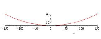
such as Newton’s iterative one. The graph above exhibits the cable shape
for a problem with L=300 ft and s=40 ft. l
is found by Newton’s method to be 287.68 ft.
where l is the horizontal tension applied to the cable divided by
the cable’s weight per unit length, s is the sag of the cable in
feet, and (L/2) the coordinate of the pole (in feet) relative to the
mid-point of the sagging cable. In this system with equal height poles,
the sag occurs at the midpoint of the segment. L is known, and either
the tension or the sag can be specified. Since l is the ratio of a tension (force in lbs) divided by the
weight density (lbs/ft), the units of l
are feet. The equation is then solved for the other parameter using a method
such as Newton’s iterative one. The graph above exhibits the cable shape
for a problem with L=300 ft and s=40 ft. l
is found by Newton’s method to be 287.68 ft.
Note that the height of the poles does not enter in here – they just need to be tall enough to accommodate the sag. - Less simplified case. Assume that the elevations
at the ends of the cable segment are different. In particular, one end
(either one) is H feet above the other end. The poles here are
still the same height, but the elevation of the land has changed by H
feet. The parameters L, l
and s are defined as before. However, in this case the bottom of
the sag occurs at a location other than the mid-point of the segment. In
particular, the minimum of the sag occurs at a point L1 from
one end and L2 from the other. L2 = L –
L1 is required. With L , H, and s specified,
there is a system of two equations to be solved for two unknowns: L1
and l. This system of
equations can be solved using Newton’s method as described in Turner’s
text. The system of equations is:

If as in the simplified case above, L=300ft, sag = 40ft, and one pole is H=15 ft above the other, the solution of the system of equations by Newton’s method yields: l = 245.95 ft, and L1 = 138.4 ft. It follows that the distance from the cable minimum to the other pole is L2 =L – L1 = 161.6 ft. The poorly labeled figure on the right shows the cable solution to this problem.
Note that the sag (40 ft) is measured from the lower end and that the
higher end is H (15 ft) above the lower one.
- Having solved the system of equations for the catenary
curve in this particular problem, we are ready to calculate the length of
the curves in these figures. These lengths are calculated by vector
integration along the curve. In the general (H¹0) case, two equations are
obtained, one for the part of the curve on the right hand side of the
minimum and one for the part on the left hand side. They are:

The overall length of the curve in this segment is the sum S = S1
+ S2. In the test case above, a cable length of
319.3 ft is needed to span the poles 300 feet apart with an elevation
difference of 15 ft, and with the 40 ft sag.
- Several data files are provided as surveyor’s data. The
following Matlab statements will read such a file extract a cell array (info)
with the data and place it in two local array variables (positionData,
altitudeData):
 The
file name is entered in single quotes (‘fname’) by the user. The names positions
and altitudes are the variable names to create the cdf file, which identify
which data to extract. The names positionData and altitudeData are
local to the calling program and can be whatever you choose. The four cdf
data files provided here are
The
file name is entered in single quotes (‘fname’) by the user. The names positions
and altitudes are the variable names to create the cdf file, which identify
which data to extract. The names positionData and altitudeData are
local to the calling program and can be whatever you choose. The four cdf
data files provided here are
|
Approximately 10 data segments, all at same elevation (H=0) |
|
|
Approximately 10 data segments, with uneven terrain. |
|
|
Approximately 1700 data segments, even terrain (H=0) |
|
|
Approximately 1700 data segments, with uneven terrain. This is the actual problem set for your final submission with the serial program.. |
|
|
Approx 17,000 data segments. |
|
|
Approx 50,000 data segments is the actual problem set for your final submission with the parallel program. |
- Programming notes (more may be added).
- Newton’s method can fail to converge; a well written Newton method will check for failure to converge and stop itself.
- There may be some solutions that are not physically meaningful, such as negative values of L, L1 or L2. A well written program would check to make sure that the lambda and L values are meaningful. You could do this as a post processing step. Devise a post processing step that checks most of the obvious characteristics besides the negative values above: sane cable lengths, height changes, etc.
- Various constants and parameters should have reasonable defaults, but also provide the user with the opportunity to specify them.
- Use the plot function frequently to examine the functions you are using and the data sets. Many errors are easy to identify with plots.
- You need to take the partial derivatives of the functions being solved to carry out the Newton method. If neither you nor your partner is sure how to do this, be sure to look it up before coding.
- Good coding practices are to be followed:
- Adequate and informative commenting throughout, including the use of and purpose of each function.
- Appropriate indentation in code and use of white space to clearly delineate logic elements.
- Comments should explain each function
- Use of white space around operators to make the lines of code more readable
- Sensible variable and function names that make code easy to understand
- Efficiency: especially regarding vector operations
- Appropriate modularization based on task components
- Only very sparing use of global variables – in most cases only as constants. Note the use of shared space within a set of nested functions however.
- Numbers should generally not appear as literals in code,
but in most cases should replaced by variables or constants.
Preliminary submission. By 11:59 PM, Friday, January 13, you are to turn in a deliverable to the “MP1PreliminarySubmission” drop box. This file is to report on the design (including modularization), author responsibilities for different components and phases of code development. It should also include rough drafts ( not yet debugged) of any modules that have been started.