Thermal Conductivity
Of Ferrofluids
Matthew Bernards
Chem E 499
6/7/01
Table of Contents Page
1.
Introduction 2
2.
Experimental Design 2
3.
Materials 6
4.
Procedures 7
5.
Early Troubles 8
6.
Determination of Steady
State Time 9
7.
Results 10
8.
Discussion 11
9.
Recommendations 13
10. Conclusions 14
11. Nomenclature 14
12. Literature Cited 15
13. Appendices
A. Apparatus 16
B. FIDAP Results 18
C. MATLAB Code – Steady State
Approximations 20
D.
Time to Steady State
Data 21
E.
Experimental Data and
Results 24
F.
Data from Trouble
Shooting Period 27
Introduction
The
uses of ferrofluids have become quite diversified in the recent years. One use for these fluids is heat
removal in transformers. The
fluids fill the internal compartments of the transformers near the coils and
help remove the heat with both conduction and convection. The purpose of this study was to
determine the thermal conductivity of pure and diluted ferrofluids, to further
understand their heat removal properties in transformers. The ferrofluid that was tested is a 45
gauss oil based fluid.
Experimental Design
Before thermal conductivity testing could begin, an apparatus for measuring the thermal conductivity needed to be designed. The basis for this design was taken from Smith [1] and his groundbreaking research measuring the thermal conductivities of several liquids in the 1930s. The original apparatus used by Smith consisted of two concentric copper cylinders with a gap of 1/64 of an inch between. The fluid of interest was placed in this gap and the entire apparatus was heated from the center copper cylinder with a high resistance wire, located in the center of this cylinder. The heat removal was accomplished by placing the entire set-up into a constant temperature oil bath. For further details on this work please refer to Reference 1, at the end of this paper.
A new apparatus was designed for this testing, patterned after Smith’s experimental set-up. The main differences consisted of upgrades in the electronics and theoretical calculations of the dimension and components. The first of these theoretical calculations was a simulation of the temperature distribution for one quarter of this apparatus. This simulation was completed with the PDE toolbox on MATLAB. This simulation represented one corner of the apparatus and it is identical for all four corners. Because it is the same for all four corners the simulation could be run for only one corner making the simulation easier to run and interpret.
In this simulation it can be seen that there are four blocks. The top three represent the inner copper cylinder, the fluid gap, and the outer copper cylinder from left to right. The large lower block represents the plexiglass cover and it was given a thermal conductivity of 0.2 W/m K. The copper blocks and fluid were assigned thermal conductivities of 400 W/m K and 0.2 W/m K respectively. The boundary conditions that were assigned to these blocks were simple approximations, to determine what the general temperature distribution trends would be. The plexiglass block was assigned adiabatic surfaces on the bottom, top, and left. The entire right hand side of the diagram was assigned a temperature equal to 0. This temperature value was also used for the top of the outer copper block. The fluid gap block was given a linear temperature distribution across it, and the other copper block was assigned a temperature equal to 1. These boundary conditions are summarized below, in Figure 1.
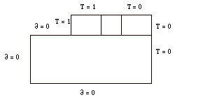
Figure 1: Boundary Conditions for Simulation
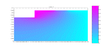 The
simulation was run under these conditions to see the overall heat distribution
trends. The purpose of this
simulation was to see if plexiglass would be an effective way to prevent the
loss of heat from the top and bottom of the apparatus. The planned calculation method included
the assumption that there was no heat loss from the top and bottom of the
apparatus, and this simulation would test that assumption. The simulation results can be seen
below, in Figure 2.
Figure 2: Simulation of Apparatus Temperatures
From
the simulation results it can be seen that there is basically no temperature
change on the lower and outer surface of the plexiglass cover. There is some temperature change on the
left side of the plexiglass, but this is only the midpoint of the apparatus and
the simulation results for the other half would be a mirror image of this. Based on this simulation, it can be
seen that the assumption of no heat loss from the plexiglass is a justifiable
one.
The
next simulation study that was completed was done to determine the dimensions
of the apparatus. This simulation
was completed with FIDAP code written by Professor Finlayson. This code simulated a two dimensional
fluid gap, modeled as a plane. The
purpose of this simulation was to determine at what point convection effects
came into play in this heat transfer process for an apparatus with a height
value of 1 and a width value of 1/64, which represented the dimensions of the
apparatus found in Smith’s work [1]. The Nusselt number was calculated by this program, for
varying Prandtl and Rayleigh numbers.
The Nusselt number is a measure of the convective heat transfer
occurring at a surface and when it is less than or equal to one, it means that
there is negligible convective heat transfer taking place within the substance
[2]. This simulation was run for
Rayleigh numbers ranging from 10-3 to 105 and Prandtl
numbers equal to 0.71, 1, 10, and 100.
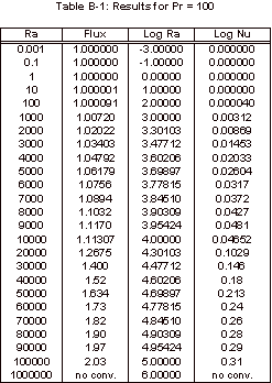
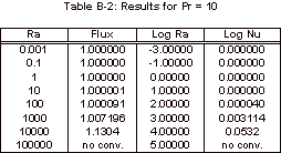
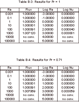
The results obtained with this simulation can be found in Appendix B and
the corresponding graph of these simulation results can be seen below, in
Figure 3.
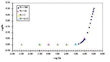
Figure 3: Nusselt Number Relationships
As
can be seen in Figure 3, the Nusselt number does not vary from one until the
Rayleigh number increases past 1,000.
It can also be noted that the Nusselt number shows no variation over the
four Prandtl numbers that were tested.
The magnitude of the Rayleigh number that is expected for our experiment
is on the order of 1, so based on this simulation it is known that there will
be relatively no convective heat transfer within our fluid sample for the
length to width ratio of 1:1/64.
The
last computer simulation that was completed was another MATLAB simulation. This theoretical calculation was
completed to estimate the steady state time it would take to achieve a certain
temperature change across the fluid.
This simulation, written by Professor Finlayson, was used to simulate a
heat flux of 1.5 W. This value and
all of the others used in the code were all approximations of the actual
experimental parameters, including an estimated thermal conductivity for the
oil. These values were used in
order to tie this simulation to our experimental work as closely as
possible. The final simulation
results can be seen below, in Figure 4 (This is revised from the original).
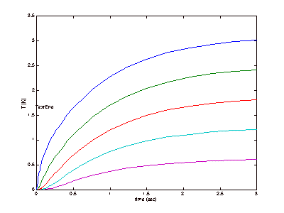
Figure 4: Steady-State Approximations
It
can be seen in Figure 4 that the apparatus will be expected to reach steady
state very quickly. It is likely,
however, that this simulation did not completely account for all of the
variables that could affect each trial run, so the time to steady state was
also tested experimentally and this will be discussed later.
The
design simulations were completed with conclusion of this final test. The apparatus was designed so that
there would be no convection effects in the fluid sample, based on the FIDAP
simulation and it was designed to have no heat losses out of the ends, based on
the results of the first MATLAB simulation. The final simulation showed that the apparatus would reach
steady state in a relatively quick manner, as seen by the extremely small
steady-state times, but this was verified experimentally as well.
Materials
The final design consisted of two concentric copper
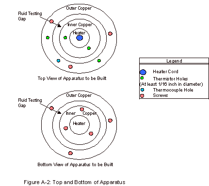
cylinders capped on the top and bottom with plexiglass. A schematic of this apparatus can be
seen in Appendix A. Although
not seen in the apparatus schematic, a 1/8 inch copper pipe was wrapped around
the outer copper cylinder. Water
was run through this pipe when operating the apparatus, in order to remove the
heat being produced by the heater.
Leakage from the fluid gap was prevented by placing two gaskets on each
cap, around the portion of the cap that protrudes into the fluid gap. These caps were held into place with
plastic screws, allowing the lids to be held on tightly, while allowing for
easy removal to clean and fill the fluid gap.
As can be seen in Figure A-2, in the Appendix, there
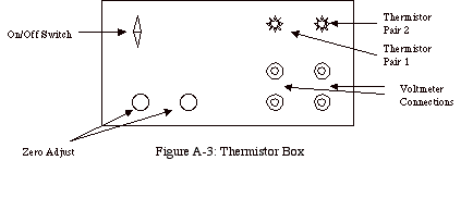
are four holes present in the top for thermistors. These thermistors are paired and allow for fairly accurate
measurements of the temperature difference across the fluid gap. This measurement is repeated, as it is
one of two key experimental values, presenting a way to determine the accuracy
of this measured temperature difference.
If the values for the two are largely different, something is not
working correctly in the apparatus and the trial results are not accurate. These thermistor measurements are
output as electronic signals, which are monitored by a voltmeter. The conversion of this voltage to a
temperature is as follows:
DT = V / 8.6 mV/oC (1)
In Equation 1, T is the temperature in Celsius and V is the voltage measured in mV. This equation is derived based on the thermistor’s power source and the resistance network between pairs of thermistors.
The other
key experimental measurement is the voltage being input into the heater. With this value the heat flux can be
calculated as follows:
q = V2/R (2)
In Equation 2, q is the heating rate in watts, V is the AC voltage input to the heater, and R is the resistance of the heater in ohms. With the current set-up, a current of about 45 volts is being used, through a heater with a resistance of 1413 ohms. This gives us a heating rate of about 1.4 watts, as calculated with Equation 2.
With
values for both the temperature difference and the heat flux, one can easily
calculate the thermal conductivity.
The equation for this is [2]:
k = q ln(r2/r1) / 2pLDT (3)
In
Equation 3, k is the thermal conductivity in W/m K, q is the heating rate in
watts, r1 and r2 are the inner and outer radii
respectively, L is the height of the apparatus in meters, and DT is the temperature difference across the gap in
Kelvin.
The thermocouple hole, which can be seen in Figure
A-2, was present in order to determine the temperature of the outer copper
block. With this temperature and
the temperature difference, the inner copper cylinder temperature could also be
calculated. This value was taken
for record purposes, as thermal conductivities vary sometimes with temperature
Procedure
The
procedure for this experiment is not overly complicated. First, the lower part of the apparatus
is assembled. This includes
placing the gaskets onto the bottom plexiglass and screwing this piece into
place. Once this has been
completed, the fluid is loaded next.
This is done using a syringe.
The fluid should be loaded slowly, around the entire gap until it begins
to come out of the top. The fluid
coming out of the top indicates that the fluid gap is completely filled. At this point the heater is inserted,
the top gaskets are put into place, and the top cap is screwed on. Next, both thermistor pairs are zeroed
using an Icell constant temperature cell.
After zeroing them, the thermistors are coated in Thermalcote and put
into place. Thermalcote is a high
thermal conductivity paste, which allows for good contact between the
thermistors and the copper. The
thermocouple is also put into place at this time. The cooling water flow is begun next, upon completion of the
assembly. Once this flow is begun,
the heater is turned on and the apparatus is allowed to heat to steady
state. Steady state is achieved
when the thermistor measurements have stabilized. Once this has occurred, the steady state temperatures and
heater voltage are recorded, completing the experimental data collection for
the calculation of that fluid’s thermal conductivity.
Clean
up for this apparatus is very similar to the setup. The thermistors and thermocouple are first removed and wiped
off. Next the top and the heater
are removed. The fluid is drained
and collected by removing the outer three screws from the bottom and pulling
the inner copper cylinder out.
Once the fluid is removed, the entire apparatus is wiped down and
cleaned, to remove any residue from the fluid that was just tested.
Early Troubles
The
first stage of the experimental testing was a verification of the accuracy of
the results that could be obtained with the apparatus. In order to do this, water was tested a
number of times. The initial
results with the water were very inconsistent and inaccurate and as a result
modifications were made in both the procedure and some of the electronics. Different procedures that were tried
included varying the length of trial runs, varying the cooling water flow rate,
and trying a constant temperature water bath as the cooling method. Over the course of these trials it was
determined that the length of trial runs seemed to be an important variable,
but the cooling water flow rate did not.
It was also determined that a constant temperature water bath did not
yield results that were any more accurate than those obtained with the cooling
water flow.
Over
the course of these initial trials, many of the apparatus’ bugs were
determined and removed as well.
One of the first improvements was the use of Thermalcote for the
thermistors. This substance
eliminated air convection in the thermistor hole, which was causing the
temperature reading to fluctuate substantially. Another improvement that was made to help eliminate drift in
the thermistors was a redesign and upgrade of their resistor system. Finally, there were a number of
improvements in the equipment itself.
One pair of thermistors continually gave extreme results and that pair
was eventually replaced. After a
time, the heater burnt out and needed to be replaced as well. The data and resulting thermal
conductivities corresponding to all of this initial work can be found in
Appendix F.
Determination of Steady State Time
One
of the simulations that was run during the design phase of the research was a
MATLAB simulation to determine the steady state time. This simulation yielded a steady state time of 1x10⁻⁵
seconds. This was seemingly
extreme, as steady state did not appear to be occurring in any of the
experimental trials for at least forty-five minutes. As a result of these contradicting results, it was
determined that the steady state behavior needed to be studied more
closely. This study was conducted
after the heater had been replaced in the trouble shooting portion of the data
collection.
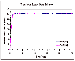 The
procedure for determining the steady state time was very basic. Temperature measurements were taken
with the thermocouple and both thermistor pairs every minute for the first five
minutes and then every two or three minutes for approximately thirty minutes
total. These measurements were
taken for one trial with water and two with octane and the results for one of
the octane trials can be seen below, in Figure 5.
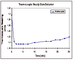
Figure 5: Steady State Trends for Octane
In
Figure 5, it can be seen that the thermistors appear to reach their steady
state values within five minutes of the start time. The thermocouple, on the other hand, shows a continual
increase in temperature over time.
These trends were seen in the other two trials as well and the results
from these two trials can be found in Appendix D, along with the data that was
collected experimentally.
Based
on the results of these experimental runs, it was determined that the
thermocouple was not a good way to determine if the temperature had reached
steady state across the fluid gap.
It was seen in all three trials that the temperature difference between
the two copper cylinders reached its steady state value long before the
thermocouple even neared its steady state value. Based on this, it was decided that trials would be run for
ten to fifteen minutes, until the thermistor readings reached their steady
state range.
Results
The
ultimate goal of this research was the determination of the thermal
conductivity of a 45 gauss ferrofluid.
The apparatus’ accuracy was tested prior to testing the ferrofluid
itself, by running experiments with octane and water. The thermal conductivity of the ferrofluid over a range of
concentrations was measured as well.
All of the average thermal conductivities can be found summarized in
Table 1, below and the corresponding data along with each individual
trial’s results can be found in Appendix E.
Table 1: Summary of Calculated Thermal Conductivities
|
Fluid* |
Number of Trials |
Thermal Conductivity (W/mK) |
Standard Deviation (W/mK) |
|
Water |
3 |
0.442 |
0.109 |
|
Octane |
6 |
0.117 |
0.005 |
|
Base
Oil |
3 |
0.106 |
0.001 |
|
80/20
Mix |
3 |
0.109 |
0.001 |
|
60/40
Mix |
3 |
0.114 |
0.002 |
|
40/60
Mix |
3 |
0.111 |
0.004 |
|
20/80
Mix |
3 |
0.112 |
0.003 |
|
45
G Ferrofluid |
3 |
0.113 |
0.001 |
*Mixtures represent Base Oil/45G mixtures.
The results obtained by varying the concentration of the mixture were also plotted to show the relationship between concentration and thermal conductivity. This plot can be seen in Figure 6, below.
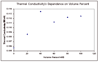
Figure 6: Concentration Dependence of Thermal Conductivity
Discussion
In order to determine the accuracy of the newly
designed apparatus two fluids were tested to see how their calculated thermal
conductivities compared to their literature values. The literature value for the thermal conductivity of octane
is 0.128 W/mK and for water it is 0.598 W/mK, both taken at 20° C [3,4].
Comparing these values to those obtained experimentally, it can be seen
that the apparatus is yielding results that are slightly lower than the
literature values.
In
looking at the calculated value for the thermal conductivity of water, it can
be seen that the results are neither accurate nor precise. There was a lot of variation in the
results obtained with the different trials, which let to an extremely large
standard deviation, 0.1 W/mK. The
inability to obtain consistent results with the water can likely be attributed
to a few things. One factor to
consider is the surface tension of the water. The fluid gap was fairly small, and it is possible that the
water did not completely fill the gap.
It is also possible that the water could have filled portions of the gap
unevenly, further affecting the results.
Another possible error associated with the water could be its
source. Tap water was used for all
of the trials and it is very possible that the water could have had any number
of contaminants in it. These could
have varied from day to day as well, resulting in further inconsistencies in
the measured thermal conductivity.
The
octane results were much more accurate than those obtained with the water. If should be pointed out that there was
one outlying trial out of the six that were run and if that trial is removed
from the average thermal conductivity calculation, the value rises to 0.119 ± 0.001 W/mK. This new average value is even closer to the
literature value and it also has a smaller standard deviation, attesting to the
consistency of the trials with the exception of the one outlying trial. These trials were also carried out over
a variety of voltages, proving that the results obtained with this apparatus
were repeatable even while varying the experimental parameters. Based on the results obtained for
octane, it was decided that the apparatus would be an acceptable method for
testing the thermal conductivity of the ferrofluid.
The
ferrofluid itself was then tested, to determine its thermal conductivity. As can be seen in Table 1, the thermal
conductivity of the 45G ferrofluid is 0.113 ± 0.001 W/mK.
This average is based on the results of three independent trials, and
based on the octane results it should be within 0.01 W/mK of the actual value.
The
final results that were obtained were the thermal conductivity’s
dependence on concentration. It
was expected that this relationship would be linear, but this does not appear
to be the case with the results from this experiment, as seen in Figure 6. With the exception of one outlying
point, it appears that this dependence is actually a second order relationship. Excel was used to fit best fit lines
and second order curves to both the original data and the data with the
outlying point removed, and the equations for these fits and the correlation
coefficients (R2) can be found on the next page, in Table 2. The trendlines themselves can be seen
with the corresponding data points in Appendix E also.
Based
on the correlation coefficients, it can clearly be seen that a second order
equation fits the results much better than the linear fit. This can be seen in the results for
both data sets. Of course the data
with the outlying point removed yield much a substantially better fit as
compared to the results that were obtained with that point included.
Table 2: Trendline Equations
|
Graph Fit |
Equation |
Correlation Coefficient |
All Data, Linear |
6´10-5 X + 0.1076 |
0.6031 |
|
All
Data, Second Order |
-1´10-6 X2 + 0.0002 X + 0.1058 |
0.8313 |
|
Point
Removed, Linear |
7´10-5 X + 0.1065 |
0.9299 |
|
Point
Removed, Second Order |
-7´10-7 X2 + 0.0001 X + 0.1058 |
0.9944 |
The
source of error that created the outlying point is uncertain. It is possible that there was an error
in making up the solution, but this is not very likely. This is due to the fact that the
calculated thermal conductivity is larger than that for the pure ferrofluid,
which is has the highest possible thermal conductivity for any combination of
it with the base oil. Another
possible source of error could have been some impurity that got into this
solution before or after it was made up.
This impurity could have caused the thermal conductivity value to be
much higher than the mixture’s actual thermal conductivity. This error source is supported by the
fact that the different trials were fairly precise, pointing to some form of
error in the mixture itself.
Recommendations
The
results that were obtained with this apparatus appear to be fairly precise and
accurate. The standard deviations
that were obtained for all of the ferrofluid trials were smaller than the
expected accuracy of the apparatus that was determined from the octane results
(0.01 W/mK). For this reason there
are very few upgrades that are recommended for the equipment. The main upgrade that is recommended is
a new method for feeding the cooling water. Currently there is a small reservoir connected by tubing to
the coil inlet. The reservoir
requires continual filling throughout the duration of the experiment and the
procedure could be simplified if a pump system or larger reservoir were
invested in. The best possible
alternative is a pumping system that could recycle the water continuously. This would prevent constant refilling
of the reservoir, aiding the operator immensely. A larger reservoir is another alternative, but this could
create problems, as it is possible that the flow rate would vary over time
depending on the liquid level in the reservoir.
Based
on the results that were obtained, there are two fluids that require additional
testing. The first fluid that
should be examined more closely is water.
Additional tests should be run with distilled water, in order to
determine why consistent results were not obtained with water initially. Distilled water would help determine if
the tap water itself was the source of the inconsistencies or if it was some
aspect of the apparatus or procedure.
The other fluid that needs to be retested is the 40 percent 45G, 60
percent base oil mixture. This was
the outlying point in the concentration graph. Retesting this mixture would result in a more accurate data
point on the concentration curve, further showing the relationship between
thermal conductivity and concentration.
Conclusions
Based
on the results obtained experimentally, this apparatus is an effective way to
test the thermal conductivity of a liquid. The apparatus appears to be accurate to within 0.01 W/mK as
seen with the octane trial results.
It can also be concluded that the thermal conductivity of the 45G
ferrofluid is 0.113 ± 0.001 W/mK, based on the experimental results. The final conclusion that can be made
from the experimental results is that thermal conductivity has a second order
dependence on concentration, as seen in the plot of these two.
Nomenclature
q =
Heating Rate [=] W
V =
Voltage [=] AC
R =
Resistance [=] W
k =
Thermal Conductivity [=] W/m K
r1,
r2 = Radius [=] m
L =
Height of Apparatus [=] m
T =
Temperature [=] oC or K
Literature Cited
1.
Smith, J. F. Downie.
“Thermal Conductivity of Liquids.” Industrial and Engineering Chemistry. Volume 22, No. 11. 1930.
2.
Incropera, Frank P. and
DeWitt, David P. Introduction
to Heat Transfer. John Wiley
& Sons, New York, 1996.
3.
Green, Don W. Perry’s Chemical
Engineers’ Handbook.
McGraw-Hill, New York, 1997.
4.
Lide, David R. CRC Handbook of Chemistry and
Physics. CRC Press, Boston,
1991.
Appendix A: Apparatus
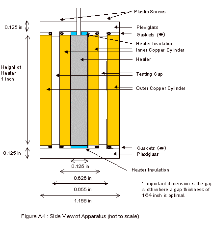
Appendix A: Apparatus
Appendix B: FIDAP Results


Appendix B: FIDAP Results
Appendix C: MATLAB Code – Steady State Approximations
%
filename run3_ht.m
% run
the transient heat transfer experiment
%
alpha is thermal diffusivity, Qdot is the heating rate
% k
is the thermal conductivity, t0 is the outer temperature
% r1
is the inner radius and r2 is the outer radius
global
a1 a2 a3 a4 r1 t0 dr n
n =
15;
r1 =
0.0079502;
r2 =
0.0083185;
dr =
(r2-r1)/n;
alpha
= 0.03;
L =
1;
Qdot
= 1.5;
k =
0.6;
t0 =
300.;
a1 =
alpha/(dr*dr);
a2 =
dr/2;
a3 =
Qdot*alpha/(k*pi*r1*L*dr);
a4 =
a3*dr/(2*r1);
y0 =
t0*ones(1,n);
tspan
= [ 0 0.00002];
[t,y]
= ode23s('rhs3_ht',tspan,y0);
plot(t,y)
xlabel('Time
(s)')
ylabel('T
(K)')
title('Fluid
Temperature Change (Q=1.5 W)')
![]()
%
filename rhs3.m
function
ydot=rhs2(t,y)
global
a1 a2 a3 a4 r1 t0 dr n
row(1)
= 2*a1*(y(2)-y(1)) + a3 - a4;
for i
= 2:n
if (i<n)
yplus
= y(i+1);
else
yplus
= t0;
end
row(i) =
a1*((yplus-2*y(i)+y(i-1)) + a2*(yplus-y(i-1))/(r1+i*dr));
end
ydot = row';