Orthogonal Collocation for Reaction-Diffusion Problems
The orthogonal collocation method has proved to be a useful method for problems of diffusion and reaction. Frequently, a first approximation gives accurate results, and it also gives insight into the solution. If desired, the higher approximations can be calculated to provide more accurate answers, and the method is suitable for bridging the gap between the regions of validity of the perturbation solutions. The orthogonal collocation method is applied here to both linear and nonlinear problems.
Consider first reaction and diffusion in a sphere when the reaction rate is linear in concentration, the Biot number for mass is large, and the temperature is constant. The problem is
![]()
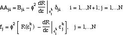
Due to the boundary condition at the origin, we use symmetric polynomials to solve this problem (link). The residuals evaluated at the N interior collocation points are
![]()
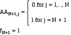
while the boundary condition requires
![]()
After the solution for c is found, the effectiveness factor is obtained using the quadrature formula.

This is more accurate than using the first derivative.
![]()
For the first approximation, we have
![]()
The solution is
![]()
and the effectiveness factor is
![]()
The solution is plotted in the figure; the values at the collocation points are shown, and the
interpolation is with the appropriate polynomial, here a quadratic function of position. For small
f the concentration is relatively constant across the catalyst pellet, whereas for larger
f the concentration dips to small values. Indeed, for the case of
f = 10, the solution is negative at the center. Since
this can't happen physically, this is one sign that more collocation points are needed and a higher
degree polynomial is necessary.

Figure 1. One-term Orthogonal Collocation Solution
For higher N, the solution is obtained numerically. Write the equations for a genera rate expression. Expand the nonlinear term in a Taylor series (for the Newton-Raphson method) and rearrange.
![]()
In the form
![]()
we need
The code is available. To see how accurate the solution is, we solve for an increasing
number of collocation points. The solution is shown in Figure 2. The solution at the collocation points for
N = 1 and 2 shows error, but for N 3 all the solutions at the collocation points lie on the curve for N
= 6. Thus, when the solution becomes steeper, you need more points.
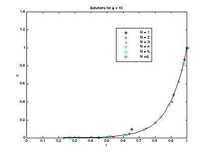
Figure 2. Orthogonal Collocation Solution for f = 10 and different N
The effectiveness factor is plotted, too, and this figure also shows the convergence with
increasing number of collocation points. This is more important for higher
f, when diffusion is slow and the reaction depletes the reactant, forming steep concentration profiles.
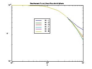
Figure 3. Effectiveness Factor for Different Approximations
Next consider nonisothermal problems. The first problem is
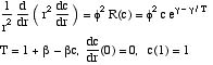
with b = 0.3, g = 18, and f = 0.5. In this case, the derivative of the rate expression is
![]()
which varies from 2.8 to 16 as c varies from zero to one. Thus, the problem is not highly
nonlinear, despite the variation of temperature. The solution is shown in the figure, and only a few
collocation points are necessary for numerical convergence to the solution of the ordinary differential equation.

Figure 4. Solution to Mild Non-isothermal Problem
Next consider the problem with b = 0.4, g = 30. Now it is difficult to obtain convergence in the orthogonal collocation method for large values of Thiele modulus. When the reaction is almost complete throughout the catalyst, the initial guess is taken as c(r) = 0 to improve the chances for convergence. In spite of that, however, solution are not always obtained with the Newton Raphson method. Furthermore, the solution oscillates near the center of the catalyst pellet if one uses the polynomial to represent the function there (the collocation method doesn't actually use the values near the center). For this problem, and harder problems, the method of orthogonal collocation on finite elements is recommended.
Take Home Message: The orthogonal collocation method is ideally suited to problems whose solution does not have extremely steep gradients. When the gradients are steep, the solution tends to oscillate, and convergence may be difficult for nonlinear problems.