Derivation of Finite Difference Equations
Elliptic equations can be solved with both finite difference and finite element methods. One-dimensional elliptic problems are two-point boundary value problems. Two- and three-dimensional elliptic problems are often solved with iterative methods when the finite difference method is used and with direct methods when the finite element method is used. So there are two aspects to consider: how the equations are discretized to form sets of algebraic equations and how the algebraic equations are then solved. This section derives the finite difference equations.
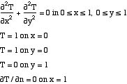
We consider a two dimensional situation so that the equation is
![]()
where Q has been added as a heat generation term (positive for generation). On the boundary we might have a flux specified, such as
![]()
or the temperature may be fixed
![]()
We illustrate the method of solution by solving the following problem.

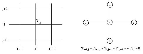
Finite Difference Notation for Two-Dimensional Problem
(right-hand figure is for x = y)
We first derive the finite difference method, and then show how to solve it on a spreadsheet. In the figure, each node is denoted by two indices, i and j. The Taylor expansions about the i-j point give the expressions for the derivatives.
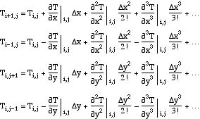
By combining these equations you can show that the differential equation at the i,jth node is given by
![]()
This represents the finite difference formulation of the elliptic partial differential equation. The boundary conditions specify the value of T on three sides; on the fourth side we use a false boundary point and write
![]()
These equations can be solved in a variety of ways: iteratively on a spreadsheet (link), iteratively in MATLAB (link), and with a direct solution in MATLAB (link).
Elliptic PDE solved with Excel.
A spreadsheet can be used to solve elliptic partial differential equations, using the finite difference method and the iteration feature of the spreadsheet. Consider heat transfer in a rectangular region. The equations have been derived elsewhere (link).
![]()
The boundary conditions specify the value of T on three sides; on the fourth side we use a false boundary point and write
![]()
To solve these with a spreadsheet we rearrange them so that we solve for the center point; as identified in the figure.
![]() (1)
(1)
This equation applies to each point in the internal of the domain. The boundary points are given on three boundaries; on the fourth we use a false boundary point and write
![]()
Thus points along the right-hand side have a modified equation
![]() (2)
(2)
To solve the problem on a spreadsheet we let each cell represent the temperature at a node. Then we place the proper equation in the cell. Let us do so for x = y. For the cells inside the boundary we put the equation (1); if cell E2 represents an interior point the equation is
![]()
The copy feature of the spreadsheet is used to copy this command to all the cells interior to the boundary. For the cells along the top, bottom, and left-hand side we put the known boundary values; we use 0.5 at the corner y = 0, x = 0. For the cells along the right-hand side we put equation (2). For example, if cell H2 is on that side the equation is
![]()
We then copy the formulas to adjacent cells.
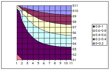
Then, let the spreadsheet program iterate until the error is small enough. Since we can watch the solution as it proceeds we can see how well the iteration process is proceeding. Once we are done, we have the temperature at each grid point, as shown below. We can either plot the solution in the spreadsheet, or put the matrix of values into a plotting program and draw contours. This method works well for simple problems. If the domain is irregular, but composed of straight sides that are all parallel or perpendicular to each other we can use the method.
| 0.5 | 0 | 0 | 0 | 0 | 0 | 0 | 0 | 0 | 0 | |
| 1 | 0.505 | 0.313 | 0.226 | 0.18 | 0.154 | 0.138 | 0.128 | 0.122 | 0.119 | 0.118 |
| 1 | 0.709 | 0.522 | 0.409 | 0.341 | 0.298 | 0.27 | 0.253 | 0.242 | 0.236 | 0.234 |
| 1 | 0.807 | 0.656 | 0.549 | 0.476 | 0.426 | 0.393 | 0.371 | 0.357 | 0.349 | 0.346 |
| 1 | 0.864 | 0.747 | 0.655 | 0.587 | 0.538 | 0.504 | 0.48 | 0.465 | 0.457 | 0.454 |
| 1 | 0.901 | 0.812 | 0.738 | 0.68 | 0.636 | 0.604 | 0.582 | 0.567 | 0.558 | 0.556 |
| 1 | 0.928 | 0.862 | 0.805 | 0.758 | 0.722 | 0.695 | 0.675 | 0.662 | 0.655 | 0.652 |
| 1 | 0.95 | 0.903 | 0.861 | 0.827 | 0.799 | 0.778 | 0.762 | 0.752 | 0.746 | 0.744 |
| 1 | 0.968 | 0.938 | 0.911 | 0.888 | 0.869 | 0.855 | 0.844 | 0.837 | 0.833 | 0.831 |
| 1 | 0.984 | 0.97 | 0.956 | 0.945 | 0.936 | 0.928 | 0.923 | 0.919 | 0.917 | 0.916 |
| 1 | 1 | 1 | 1 | 1 | 1 | 1 | 1 | 1 | 1 | 1 |
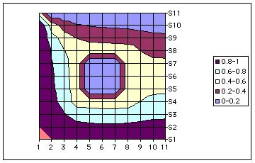
For example suppose there was a hole in the center of the domain, and the temperature was kept at a value of 0.5 there. Then we would take out the equations in the hole, place the value 0.5 on the boundary of the hole, and redo the solution. The result is shown in the table and figure. As in all the problems we must resolve the problem with more grid points to confirm the accuracy of the solution. We can easily add the heat generation term, and we can make it a function of position as well.
| 0.5 | 0 | 0 | 0 | 0 | 0 | 0 | 0 | 0 | 0 | 0 |
| 1 | 0.5 | 0.306 | 0.222 | 0.188 | 0.173 | 0.164 | 0.155 | 0.14 | 0.13 | 0.126 |
| 1 | 0.695 | 0.5 | 0.394 | 0.355 | 0.34 | 0.33 | 0.315 | 0.277 | 0.253 | 0.245 |
| 1 | 0.779 | 0.606 | 0.5 | 0.5 | 0.5 | 0.5 | 0.5 | 0.399 | 0.359 | 0.349 |
| 1 | 0.814 | 0.646 | 0.5 | 0.5 | 0.459 | 0.437 | 0.431 | |||
| 1 | 0.831 | 0.665 | 0.5 | 0.5 | 0.5 | 0.5 | 0.5 | |||
| 1 | 0.845 | 0.681 | 0.5 | 0.5 | 0.541 | 0.563 | 0.569 | |||
| 1 | 0.867 | 0.715 | 0.5 | 0.5 | 0.5 | 0.5 | 0.5 | 0.602 | 0.641 | 0.652 |
| 1 | 0.908 | 0.812 | 0.716 | 0.685 | 0.676 | 0.676 | 0.687 | 0.724 | 0.748 | 0.755 |
| 1 | 0.954 | 0.909 | 0.868 | 0.849 | 0.841 | 0.841 | 0.847 | 0.86 | 0.871 | 0.874 |
| 1 | 1 | 1 | 1 | 1 | 1 | 1 | 1 | 1 | 1 | 1 |