Derivation of Implicit Methods

By evaluating f(y) at the new time, using yⁿ⁺¹, it is possible to derive implicit integration methods. Implicit methods result in a nonlinear equation to be solved for yⁿ⁺¹ so that iterative methods must be used. The backward Euler method is a first-order method.

Errors are proportional to t for small t. The trapezoid rule is a second-order method.

Errors are proportional to t² for small t. When the trapezoid rule is used with the finite difference method for solving partial differential equations it is called the Crank-Nicolson method. The implicit methods are stable for any step-size, but do require the solution of a set of nonlinear equations, which must be solved iteratively. The set of equations can be solved using the successive substitution method or Newton-Raphson method. See Ref [Bogacki, et al., 1989] for an application to dynamic distillation problems.

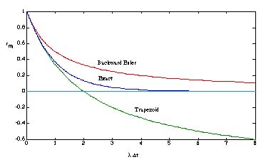
When the ratio r_mq is calculated, if it is always less than +1 and greater than -1 then the method is stable for any step size. This is the case for the Backward Euler method and the Trapezoid method, as shown in the figure.

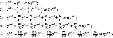
The best packages for stiff equations (see below) use Gear's backward difference formulas. The formulas of various orders are [Carnahan, et al., 1969; Gear, 1971]

Implicit methods are available for MATLAB, too. For example, one stiff package is called ode15s. To solve the turbulence model we would replace the statement

[t,u] = ode45('turb',tspan,u0)

with

[t,u] = ode15s('turb',tspan,u0)

If the problem is stiff then such methods may be needed.

Take Home Message: Implicit methods are able to solve stiff problems. However, to do so, sets of nonlinear equations must be solved at each time step. Thus, they can take a long time. If an explicit method will work, it is often more accurate, but implicit methods are needed for some problems.