Extrapolation & Errors
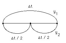
Richardson extrapolation can be used to improve the accuracy of a method. Suppose we step forward one step t with a p-th order method. Then redo the problem, this time stepping forward from the same initial point, but in two steps of length t/2, thus ending at the same point. Call the solution of the one-step calculation y1 and the solution of the two-step calculation y2.
Then an improved solution at the new time is given by
![]()
This gives a good estimate provided t is small enough that the method is truly convergent with order p. This process can also be repeated in the same way Romberg's method is used for quadrature.
To prove this result, take a p-th order method. The numerical solution, called y1n+1, after one step has an error that is proportional to tp.
![]()
Back up and start from the same point, this time taking two steps of size t/2. Then the numerical solution, called y2n+1, has an error that is proportional to (t/2)p.
![]()
From the numerical results one knows y1n+1, y2n+1, and t. Thus solve these two equations for c and yexn. The result gives
![]()
Now this value will not be the exact solution because the error expressions have neglected terms higher power than tp. However, this extrapolation can improve the accuracy considerably.
Apply this process to solve
![]()
Euler's method is
![]()
Results were obtained for y(1) using several different t: 0.2, 0.1, and 0.05.
| Ćt | y(1) | error in y(1) |
| 0.2 | 0.32768 | -0.0402 |
| 0.1 | 0.3486784 | -0.0192 |
| 0.05 | 0.3584859 | -0.0094 |
| extrap. | 0.3682934 | 0.00041 |
Since Euler's method is first order, the extrapolation goes as
![]()
where, for example, y2 is the answer obtained with t = 0.05 and y1 is the less accurate answer obtained with t = 0.1. Here that gives y = 2 x 0.358485922 0.3486784 = 0.3682934. The exact answer is exp (1) = 0.367879. Using the extrapolated answer gives an actual error of only 0.0004, whereas the solution with smallest time step had an error of 0.00939, or almost 23 times larger. By using these extrapolation techniques we can assess the numerical error. We can also plot the result versus t and, if t is small enough for the asymptotic results to be valid, we should get a straight line. This is what is seen in Figure 1. Note, however, that this proportionality only holds for small enough t, and the 'small enough' usually has to be found by trial and error.
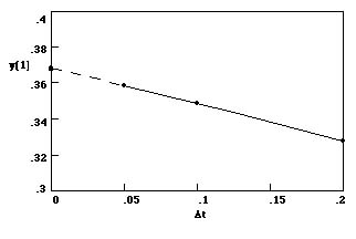
Figure 1. Values of y(1) plotted versus t
In this case we know what the exact solution is, and we can calculate the actual errors, which are listed below. If these are plotted we also get a straight line, as seen in Figure 2.
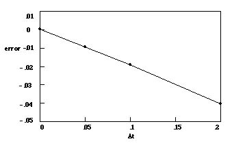
Figure 2. Error in Computing y(1) using Different t
Take Home Message: If you use a method with a fixed step size, it is easy (and well worth the effort) to solve the problem with at least three step sizes and extrapolate to zero step size.