Explicit Solution with MATLAB

In MATLAB we merely call a subroutine which carries out the integration. We need to prepare an M-file which defines the equation and then call the subroutine (ode45) to do the integration. This method may seem mysterious at first because you call a subroutine, which in turn calls your M-file. Thus the commands you give and the M-file are somewhat disparate. The process is illustrated using a single, simple differential equation:

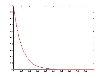
Integrate this equation from t = 0 to t = 1. The exact solution can be found by quadrature and is

To use MATLAB we first construct an M-file that defines the equation.

% filename rhs.m
function ydot=rhs(t,y)%compute the rhs of eqns.
%for any input values t, y
ydot = -10*y %compute rhs

The function needs to be tested. To do this, issue the command

q = rhs(0.2,3)
ydot = -30
q = -30

When y = 3, the value of the right-hand side should be ­30, so the program is correct.

Next create an M-file that is the script to run the problem. These commands can also be typed in the command window, but when you have several commands that you will use over and over it is more convenient to create a script that can run all the commands with one message from you.

% filename simple.m
ini=1.; %set the variable ini to 1.
y0=ini; %set the initial condition to ini
t0=0; %set the initial time to zero
tend=1; %set the final time to 100
tspan=[t0 tend]; %need to use it in this form in MATLAB 5.
[t,y]=ode45('rhs',tspan,y0)%call the routine ode45
plot(t,y) %plot the solution

The results give a table of values for t and y and a figure.

t =	0.	0.0078	0.0268	0.0460	0.0659	0.0865	0.1080	...
y =	1.0000	0.9248	0.7647	0.6314	0.5175	0.4209	0.3395	...

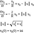
Next consider the following two ordinary differential equations, which are a model of turbulence.

We first make an M-file named turb.m

function udot=turb(t,u)
%compute the rhs of eqns. for any input values t, u
global R%make R available in function
unorm = sqrt(u(1)*u(1)+u(2)*u(2)); %calculate intermediate value
udot(1) = -u(1)/R + u(2) - unorm*u(2); %compute first rhs
udot(2) = -2.*u(2)/R + unorm*u(1); %compute second rhs
udot = udot' %converts a row vector to the
%column vector needed by ode45 (below)

This M-file needs to be checked. This can be done by calling the function from the command line, but the way this is done depends on your version of MATLAB. First, in the command mode make the variable R global and set it equal to 25.

global R%make R available in functions that use global R
R=25 %Set R to 25

Next call the subroutine for specified values of u. It is helpful to remove the ';' in the M-file so that the results of each step of the calculation will be printed.

turb(0.2,[2 3]
unorm = 3.6056
udot = -7.897
udot = -7.897 6.971

In addition, it is useful to make sure all variables entered the routine correctly. We have done that here, since the right-hand sides are correct, but in more complicated problems it is useful to actually print the values inside the routine. This can be done by adding to the M-file:

R [or disp(R)]

which would give the print out (when the subroutine was called)

R = 25

Naturally, once the M-file is checked, all ';' are put in and the extra print statements are removed.

If the command shown above does not work with your version of MATLAB, use the feval function. This will require that you take out the t in the M-file function definition. For example, make the M-file start with

function udot=turb(u)

and issue the command

feval('turb',[2 3])

After checking, put the t back into the M-file.

To integrate the equations we need the following commands. The text following the '%' sign gives explanations (which are not executed by MATLAB). These are the commands to integrate the equations. (The results will be interspersed with these commands.

ini=1.e-7; %set the variable ini to 1.e-7
u0(1)=ini; %set the initial condition for u₁ to 1.e-7
u0(2) = ini; %set the initial condition for u₂ to 1.e-7
t0=0; %set the initial time to zero
tend=100; %set the final time to 100
tspan = [t0 tend]] %set the time interval from t0 to tend
[t,u]=ode45('turb',tspan,u0) %call the routine ode45 %(transparent to user)

The output of the program will be a vector of times t and a matrix of u, giving u(:,1) and u(:,2) at each time. Then the norm is calculated.

nn=size(u); %find the dimensions of u (18 x 2, e.g.)
n=nn(1); %set n = the first dimension of u
for i=1:n %for n times, compute the norm at each time
un(i)=sqrt(u(i,1)*u(i,1)+u(i,2)*u(i,2)); %calculate the norm
end

This is the output. The times at which solutions are obtained are these.

t =
0
0.7812
7.0312
...
88.2812
94.5312
100.0000

These are the solutions at the above times.

u =

1.0e-05 *

0.1000	0.1000
0.1715	0.0939
0.5382	0.0570
...	...
0.0743	0.0001
0.0582	0.0001
0.0470	0.0000

This command transfers the vector un to the new vector u2 for plotting purposes.

»u2 = un
u2 =
1.0e-05 *

0.1414
0.1955
0.5412
...
0.0743
0.0582
0.0470

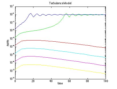
This command plots two curves, u1 versus t and u2 versus t as a semilog plot, with the y-axis being the log axis.

»semilogy(t,u1,t,u2)

The following commands label the axes.

»Title('Turbulence Model')
»xlabel('time')
»ylabel('norm')

The solution comes back as a matrix, with the first entry being the index number corresponding to the time, and the second index giving the variable. The variable t has the same number of entries. Thus, we could plot just one of the variables by saying

plot(t,u(:,1))

We could also plot one variable versus another by saying

plot(u(:,1),u(:,2))

Try it and see what you get! (The best results are for ini = 0.01 or so.)

Take Home Message: To use MATLAB to integrate initial value problems, create an M-file that defines the right-hand side, set the initial conditions and the time interval and call ode45.