Boundary Layer Flow
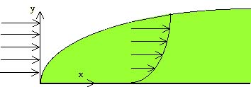
When a fluid goes past a solid object at high speed, but the flow is still in the laminar regime, a boundary layer is formed because the fluid velocity must be zero at the solid object (which is presumed stationary), and the velocity rises quickly from zero at the solid object to the mainstream velocity a bit away from the solid. A typical situation is shown in the figure.
To analyze this situation, one makes order of magnitude estimates of the terms in the Navier-Stokes equations, and ignores the ones that are small. This analysis is done in textbooks and is not repeated here (ref). After doing this analysis, however, the problem is reduced to the following differential equation and boundary conditions.
![]()
This is the Blasius equation, with a slight revision due to Deen (ref). The original Blasius equation had a 2 in front of the nonlinear term, and that number is subsumed by Deen (ref) into the definition of the stretched coordinates. The function f(h) is the stream function, and the velocity, divided by the far-stream velocity is given by its derivative.
![]()
The stretched coordinate is, in physical terms
![]()
where
![]()
One item of interest is the shear stress on the wall, which is given by
![]()
in this notation. The key number to be derived from the solutions is the value of
![]()
The exact value is 0.332. We solve this problem using an initial value technique and the integral method, one of the Methods of Weighted Residuals.
Take Home Message: The boundary layer formulation has reduced the partial differential equation to an ordinary differential equation, which can be solved easily with a variety of methods..