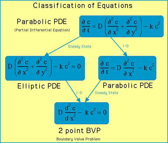
Classification of Equations
Mathematical models of chemical engineering systems can take many forms. These can be sets of algebraic equations, differential equations, or integral equations, for example. Consider the figure, which illustrates the relationships of the equations.
Starting with a two-dimensional, time-dependent diffusion-reaction problem, one can obtain an elliptic partial differential equation when assuming steady state (no time dependence). One can obtain a parabolic partial differential equation in one-dimension for cases in which there is no variation in one of the directions. The elliptic equation can be simplified to a two-point boundary value problem when only one dimension is important. The parabolic partial differential equation becomes the same two-point boundary value problem when steady state is assumed. Other examples are given below.
Algebraic Equations, example one, from thermodynamics. The perfect gas law is a linear equation for the specific volume when the pressure and temperature are known.
![]()
However, at high pressure, the perfect gas law may not represent reality, and a cubic equation of state, common to Redlich-Kwong equations, will be used.
![]()
In this case, when the pressure is known, all the coefficients are known but we are left with a cubic equation for the specific volume. This is, therefore, a nonlinear equation, but it is still algebraic.
The solution is the value of ![]() .
.
Algebraic Equations, example two, from chemical reaction engineering.
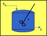
Consider a stirred tank reactor, shown in the figure. The flowrate coming in and out is the same (hence the total volume of fluid in the vessel remains constant), and in steady state a mass balance gives the change of moles in the vessel equal to the rate of generation (or removal) of the chemical in the vessel. A typical equation governing the concentration out of the reactor is
![]()
where one knows F, the flow rate; V, the volume; Vm and Km, constants in the reaction rate expression; and cin, the inlet concentration. Excel and Matlab are convenient software packages to solve this nonlinear equation.
The solution is the value of c
Algebraic Equations, example three, from chemical reaction engineering. If more than one variable is present, for example three different chemical species, with the following reaction
![]()
and reaction rate
![]()
then there are multiple nonlinear equations to solve.
![]()
The solutions are the values of c1, c2, and c3.
Ordinary differential equation - initial value problem, example one. If we model a stirred vessel but the concentration of some chemical in the inlet changes in time, the appropriate model is an ordinary differential equation.
![]()
In this case, the solution to the differential equation gives the outlet concentration versus time. Also, the problem is linear in the concentration (if you double the inlet and initial concentrations, the concentration throughout all time is also doubled). This equation is called an ordinary differential equation initial value problem (ODE-IVP) - because the solution proceeds from some initial conditions. It is an ordinary differential equation because the dependent variable (concentration) depends on only one independent variable (time).
The solution is: 
Ordinary differential equation - initial value problem, example two, from chemical reaction engineering.
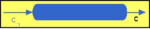
Consider the plug flow reactor shown in the figure. The tube might be filled with catalyst particles. The mass balance on a reactant might be
![]()
In this case the problem is an ordinary differential equation, as an initial value problem.
The solution is: 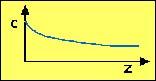
There might be a mass transfer resistance between the fluid and the catalyst so that the concentration in the fluid and in the catalyst are different. In that case, the equations governing the reactor are
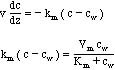
The first one is an ordinary differential equation for c, but one needs cw. The second one is an algebraic equation relating c and cw. This is a differential-algebraic problem and involves both oridinary differential equations and algebraic equatins.
The solution is 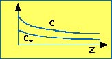
Ordinary differential equation - boundary value problem, example one, from heat transfer. Another type of problem is that for heat transfer through a slab. One side of the slab is kept at one temperature, and the other side of the slab is maintained at another temperature. The governing equation is
![]()
with boundary conditions
![]()
This is also an ordinary differential equation, because the dependent variable (temperature) depends on only one independent variable (position, x). It is called a two-point boundary condition because the boundary conditions are located at two different locations, and the solution at any position is influenced by both of them.
The soluion is: 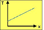
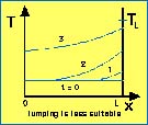
Ordinary differential equation - boundary value problem, example two, from chemical reaction engineering. If the plug flow reactor is run at low flow rates, it is possible that axial dispersion will be important. In that case, the model of the reactor is
![]()
Now, however, the boundary conditions are at both ends.
![]()
Thus, this is a two-point boundary value problem, too.
The solution is: 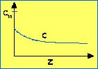
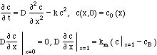
Parital differential equations - in one space dimension, example one, from mass transfer. If heat transfer takes place in a slab, but starting from one temperature profile, after which the temperature on one side changes, we get a parabolic partial differential equation
![]()
![]()
The equation for unsteady diffusion in one dimension is similar.
![]()
The temperature (or concentration) depend on two variables (time and spatial position), so that they are partial differential equations. The distinguishing characteristic of a parabolic equation is that it is evolutionary (like initial value problems you start from somewhere), but has characteristics of two-point boundary value problems (the solution depends on both boundary conditions). In fact, usually for long times the parabolic equation becomes a two-point boundary value problem, since the time derivative becomes zero.
The solution is: 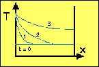
Parital differential equations - in one space dimension, example two, from mass transfer. An example hyperbolic partial differential equation is the one governing flow into a packed bed in which a species contained in the inlet can be absorbed onto the packing. One version of that is
![]()
A distinguishing characteristic of a hyperbolic equation is that the solution can move along in waves, and even shocks can form and move along 'intact'. The example equation is a partial differential equation because the dependent variable (concentration) is a function of two independent variables, time and spatial position.
The solution is: 
Parital differential equations - in two space dimensions, example one, from heat transfer. Heat transfer in a flat domain is governed by Laplace's equation
![]()
with boundary conditions all around the domain.
![]()
This equation is elliptic, and the primary distinguishing characteristic is that the solution at any point is influenced by the boundary conditions on the entire surface. The temperature at any point is a possible function of two variables, making it a partial differential equation.
The solution is: 
Partial differential equations - in two space dimensions, example two, from chemical reaction engineering.
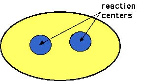
Suppose one has a multi-dimensional problem as illustrated. In the reaction centers reaction takes place, but in the surrounding (intracellular space) only diffusion occurs. The equations in the intracellular space are
![]()
with a boundary condition at the outer boundary.
![]()
For the special case in which the reaction centers are all at the same concentration, the following condition balances the diffusive flux up to the reaction center with the mass transfer flux through a membrane (or other mass-transfer limiting device) on the outer section of the reaction center.
![]()
Then, to find the cellular concentration when reaction is taking place, one also solves
![]()
Thus we end up with a complicated partial differential equation system, combined with algebraic equations.
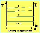
Model simplification, example one, from heat transfer. Suppose we are solving the heat transfer problem
![]()
![]()
A typical solution is shown in the figure.
Sometimes a variable doesn't change much in space, even though we have an equation governing that change. In that case, it might be useful to assign just one value to the variable, for all space (as we did above for the cellular concentation). If the thermal conductivity is so large that the temperature doesn't change much in the x-direction, as in the figure, the equation is integrated over space, and it is possible to turn it into an ODE-IVP, sometimes called a lumped parameter model.
Integrate over the volume.
![]()
The integral on the right-hand side can be written in terms of the boundary conditions.
![]()
The integral on the left-hand side is written as
![]()
where <T> is the average temperature over the range x = 0 to L, and this temperature is essentially constant, and equal to T(L,t). Then the model becomes
![]()
Now we only know the average temperature, averaged over the thickness L; we are basing the model on our intuition that the temperature is relatively constant over that region, in which case the average temperature is the same as the constant temperature.
Model simplification, example two, from chemical reaction engineering. If one has a reaction-diffusion problem governed by these equations
the integration over the volume gives
![]()
Application of the boundary conditions makes this
![]()
The lumper parameter problem is
![]()
Again, this is an adequate simplification provided the concentration c does not vary much over the thickness L.
Integral Equations. Radiative heat transfer may lead to integral equations.
![]()
There is a correspondence between integral equations and initial value problems and two-point boundary value problems, and this correspondence is described in the sections on integral equations (link).
Eigenvalue problems. Finally, the method of separation of variables to solve partial differential equations (link) can lead to eigenvalue problems. One example of an eigenvalue problem is
![]()
In this case, one solution is obvious u = 0. However, for certain values of l, non-zero solutions are possible. Those values of l are called eigenvalues, and the corresponding solution is called an eigenvector. There may be infinitely many eigenvalues and corresponding eigenvectors.
Navier-Stokes equations. In vector form, the Navier-Stokes equations are
![]()
where the first term is the inertial terms, the next term is the pressure gradient, the next term is the acceleration due to gravity, and the last term is the viscous term. The continuity equation for an incompressible fluid is
![]()
The field of numerical analysis that solves these equations is called computational fluid dyanamics (CFD). This book describes some of the methods used in commercial codes to solve these equations.
There are of course other problems you might be asked to solve: calculate an integral (called a quadrature, link); interpolate a function between the data points (link); and estimate the parameters than make your model fit experimental data (link). These, and other topics, are covered in these lessons.
Take-home Lesson: You must learn to identify the type of equation, because the equation type determines the method used to solve it.