Problem II Solved with Excel using the 'Solver'

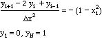
The problem to be solved is

The finite difference formulation of this problem is

Rearrange the differential equation to the following form.

The goal is to make this equation equal zero for all i = 2, . . . , N­1 by changing the values of y. Thus we want to

by changing y₂, y₃, . . . , y_N-1.

This minimization is carried out using the 'Solver' Add-on in Microsoft Excel. Consider the grid shown in the Figure.

The first row is reserved for the value of y at each grid point. The left-most cell is the value of y at the first point, and the right-most cell is the value of y at the last point. Since these values are known we simply insert the known values in the cells. The second row is reserved for the equations; we want them all eventually to be zero.

It is convenient if we define some quantities, first, though, to simplify the algebra. Let the third row represent the value of x at the node i. The value of x is placed in cell A5; first use 0.5. The first value of x, 0, is placed in the cell A3. Then the equation is written in cell B3 and copied to the right.

B3: = A3+$A$5, copied to the right

The $A$5 insures that when the cell formula is copied to the right, the next cell has B3+$A$5, then C3+$A$5; in other words, the A5 location is absolute and is not incremented during the copying. Once this is done, the third row should show the values 0, 0.5, 1.0.

Since the term involving x and x is used constantly, its value is placed in the fourth row. The first column uses:

A4: = $A$5*$A$5*(1­A3*A3)/2., copied to the right

Then the formulas for the cells involving y_i are simply:

B2: = abs(0.5*(A1 + C1) ­ B1+ B4), copied to the right (not necessary since C1 = 1.0).

Choose Tools, then the Solver Add-in (this is not installed automatically, so you may have to install it). Choose Options, and set the maximum number of iterations to 500, and the tolerance to 10^-6. Then 'Set the Target Cell' to D2, which you want to make zero by 'Changing Cell' B1. After you choose 'Solve' the spreadsheet should look like this.

	A	B	C
1	0	0.59374969	1
2		3.0903E-07		3.09028E-07
3	0	0.5	1
4	0.125	0.09375	0
5	0.5

How do we check our work? First, we make sure that the numbers we put in are correct. We check cell A5, which has the value of x; 0.5 is correct. Then we check the third row, which shows the location of the grid points. They should be x = 0, 0.5, 1.0, and these are correct. We then check the fourth row. Since we copied the formula, we only need to check one cell. For cell B4 the value should be

and this checks as well. Lastly we check the cell B2 by inserting the numbers from cells A1, B1, C1 and B4. We get

Since these calculations agree, we conclude we have set the spreadsheet up correctly. There is one final check that can be done. Notice in the formulas that if we set x = 0, then the fourth row is all zero. This is equivalent to saying there is no heat generation. Under those circumstances the solution to the problem is a straight line. Set cell A5 to 0 and see. The third row is zero, too, but as long as the fourth row is zero, the third row is essentially not used. Since we get the straight line we have added confidence in our solution.

Next do the same thing with a x = 0.25. Copy the spreadsheet for x = 0.5, then expand it to cover the number of cells for x = 0.25. Check it as before. The objective function is now in column F (in the example in F11), and the equation is =sum(B11:D11). The target cell is F11, and the cells to be changed are in cells B10:D10. The spreadsheet results are shown in the Table.

	A	B	C	D	E	F
10	0	0.54668777	0.85900061	0.983845607	1
11		3.9747E-08	1.6075E-05	0.000342199		0.00035831
12	0	0.25	0.5	0.75	1
13	0.125	0.1171875	0.09375	0.0546875	0
14	0.25

The solution is not very good. In fact, one of the equations is not satisfied and has an error 0.00034. It is difficult to get the 'Solver' to do a better job than this. Since this is a minimization problem, and there are three variables to vary, and only one objective function, changes in one variable may not make much difference in the objective function, and this makes it difficult to find the true minimum (here the objective function should be zero). Thus, this is not a very good way to solve boundary value problems.

Take Home Message: When solving sets of equations from finite difference methods, using the 'Solver' may not work.