(Courant and Hilbert, 1953) The calculus of variations is a generalization of the calculus of functions. If we are given a function f(x,y,...), defined in a closed region A, we might ask for the point in the region (x₀, y₀, ...) at which the function f(x₀, y₀, ...) is a maximum or minimum. The theorem of Weierstrass says that "Every function which is continuous in a closed domain A possess a largest and smallest value in the interior or on the boundary of the domain." If the function is differentiable and attains its minimum in the interior of the region, then the derivatives of f(x,y,...) vanish with respect to each variable at the point (x₀, y₀, ...); the gradient of the function f is zero there.

In the Calculus of Variations, we expand these concepts to include functionals. In real analysis, a function is a mapping from the real line to the real line: specify a value of x and find the function f for that x. In the Calculus of Variations, the mapping is from a function to the real line. We want the extremal of the functional rather than the function, and we consider all possible functions in some class to find that extremal rather than all possible positions (x₀, y₀, ...) in the domain A. What is the function that minimizes the functional? Naturally, the function must come from a space of functions, which must be defined for each problem, just as the minimum of a function is for the space of positions in a domain A.

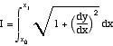
A simple example of a functional is the integral representing the length of a curve connecting the points (x₀, x₁). The length, a real number, is given by

⁽¹⁾

The length depends on the function y(x), which may be taken as a continuous function with piecewise continuous derivatives (which defines the space). We can then ask for the minimum length of the curve connecting the points y((x₀) = y₀ and y(x₁) = y₁. The answer is, of course, a straight line. Below we see how that result is derived as the solution to the "Euler equations".

The Calculus of Variations is first explained for a single variable. Take the variational integral as

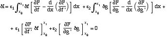
By expressing the function as the extremal plus a variation,

the variational integral becomes a function of the variables e.

One then differentiates the integral with respect to the variable e.

We define the first variation as

and set it to zero.

Next one integrates terms by parts to derive the Euler equations and natural boundary conditions.

The Fundamental Lemma of the Calculus of Variations says that if the following integral is zero for arbitrary h in a class of functions, then the term in the brackets must be zero.

The argument is that if G is non-zero anywhere, h can be set equal to G there, and the result would be positive, contradicting the condition. Here the variation is to be zero when df is chosen arbitrarily, and thus the coefficients in each brackets must be zero.

One thus obtains a set of differential equations with natural boundary conditions that govern the extremal. The argument is that if the integral is made stationary with respect to variations which satisfy this equation, with no prescribed condition on the boundaries, then it is certainly stationary with respect to a smaller class of functions which do take specific vales on the boundaries (and

hence whose variation on the boundary is zero). This gives the Euler equation. Note also that if the variation is zero on the boundary, then the natural boundary condition is not needed. What we have done is made a connection between minimizing an integral and solving a differential equation.

For Eq. (1) we get

The Euler equation is then

Note that the straight line

satisfies the Euler equation, as it should.

We next introduce a direct method of finding the extremal, as a way of solving the differential equation. Take a specific example and make stationary the functional

among all functions which satisfy y(1) = 1. Here

and the Euler equation is

The natural boundary condition comes from

Here

We don't use the condition at x = 1 so that

and the natural boundary condition is

We expand in a set of functions

where each of the y_i(1) = 0. Then the trial function y(x) satisfies the boundary condition y(1) = 1 for all values of the constants {a_i}. The first derivative is

and the first derivative squared is

The variational integral is then

Take the derivative of this integral with respect to the coefficients a_k and set it equal to zero.

But the first and second term are really the same thing, and we get

We can write this in the form

where

Note that we can calculate the matrices provided the basis functions, {y_i(x)}, are specified. The matrix equation is then solved for the coefficients , {a_i(x)}, to give the solution. We continue this process, in theory, until n -> , but in practice we stop with an n big enough that the solution no longer changes. At n -> we have made the variational integral stationary among all possible changes in the function if the sequence of functions, {y_i(x)}, is complete. In that case we have found the extremal, and it satisfies the Euler equation and natural boundary conditions. Here those are

There are some tricky points, though, as to whether the trial solution converges to the solution when the variational integral converges to its minimum or greatest lower bound. Usually we ignore those, but they can be important in special cases.

Courant and Hilbert (Vol. I, p. 173) give a good description why a variational problem may not have a solution. "In the theory of ordinary maxima and minima the existence of a solution is ensured by the fundamental theorem of Weierstrass. In contrast, the characteristic difficulty of the calculus of variations is that problems which can be meaningfully formulated may not have solutions ­ because it is not in general possible to choose the domain of admissible functions as a 'compact set' in which a principle of points of accumulation is valid. A simple geometric example is the following: Two points on the x-axis are to be connected by the shortest possible line of continuous curvature which is perpendicular to the x-axis at the end points. This problem has no solution. For,

the length of such a line is always greater than that of the straight line connecting the two points, but it may approximate this length as closely as desired. Thus there exists a greatest lower bound but no minimum for admissible curves."

Courant and Hilbert (Vol. I, p. 176) also describe the fact that the minimizing sequence may not converge to the solution. "We may now expect the resulting minimizing sequence [of the expansion y = S_ia_i y_i(x)] to converge to the desired solution. Unfortunately things are not so simple,... In general we can only state that the values of [the variational integral] obtained in this way converge to the desired greatest lower bound or minimum. Whether the minimizing sequence itself converges to the solution is a difficult theoretical question which has to be investigated separately." Courant and Hilbert (Vol. I, p. 183) give an example in which the minimizing sequence converges to the solution, but the derivative of the minimizing sequence does not converge to the derivative of the solution.

When there are several functions, a variational problem can still be expressed. For example, find the functions f(x) and g(x) that minimize the integral

By expressing the function as the extremal plus a variation,

the variational integral becomes a multi-valued function of two variables, e₁ and e₂.

One then differentiates the integral with respect to the variables e₁ and e₂.

We define the first variation as

and set it to zero.

Next one integrates terms by parts, just as before, to derive the Euler equations and natural boundary conditions, which are now more complicated.

Since the variation is to be zero when any one of the functions df or dg are chosen arbitrarily, the others being zero, the coefficients in each brackets must be zero.

One thus obtains a set of differential equations with natural boundary conditions that govern the extremal.

In addition to the Euler equations giving the differential equation that is satisfied by the extremal, there are Legendre conditions which provide necessary conditions that the extremal make the variational integral a minimum or maximum. These can be derived by taking the second derivative of I(e) with respect to e. The necessary condition for a minimum is

For a detailed proof, see Courant and Hilbert, Vol. I, p. 215.

Variational principles can also be defined for problems with constraints. Here we just outline the approach. An isoperimetric problem is to minimize the variational integral subject to a subsidiary condition like

One then writes the variational integral in terms of the combined function F + l G. The Euler equation is derived, and it contains the constant l.

The value of l is determined by the integral expression for K, i.e. c.

If we have a variational integral depending on two functions,

and the two functions are restricted by a second equation,

then one constructs the variational principle for the combined function F* = F + l G. Now, however, the l is a function rather than a constant.

If the constraint is a differential equation,

one does the same thing: write a variational principle for the combined function F* = F + l G.