LU decomposition

The most efficient way to solve a set of linear equations is to use an LU decomposition, since then one can solve for multiple right-hand sides with little extra work. This decomposition is essentially a Gaussian elimination, arranged for maximum efficiency. The LU decomposition is done by calculating in turn

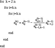
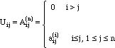
Then two matrices are formed. The U = A⁽ⁿ⁾ is defined as

The L is defined as

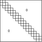
The U is upper triangular; it has zero elements below the main diagonal and possibly non-zero values along the main diagonal and above it (see the figure). The L is lower triangular. It has 1 in each element of the main diagonal, values below the diagonal, and zero above the diagonal (see the figure). It is possible to show (Ref.)

A = L U

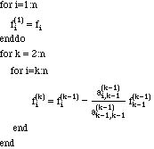
Then to solve the original problem we solve in two steps:

L y = f, U x = y, A = L U solves A x = L U x = f

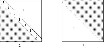
Structure of the L and U matrices

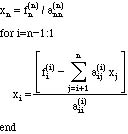
Each of these steps is straightforward, since they are upper triangular or lower triangular. The solution is performed using the equations

When f is changed the last steps can be done without recomputing the LU decomposition. Thus multiple right-hand sides can be computed efficiently. The number of multiplications and divisions necessary to solve for m right-hand sides is

The actual algorithm used will be different for parallel computers.

If

no pivoting is necessary. For solving two-point boundary value problems and partial differential equations this is often the case.

Structure of Block Tri-diagonal Matrix

A block tri-diagonal matrix (see the figure) frequently arises when solving multiple differential equations, either two-point boundary value problems or partial differential equations. When solving several simultaneous equations it is important to arrange the unknowns in a particular way to achieve the block tri-diagonal form of the matrix and the resulting efficiencies. Suppose we are solving for two unknowns, say temperature and concentration, and that we have a value for each at each node, i=1 to n. Thus we have unknowns {c₁,c₂,...c_n, T₁,T₂,...,T_n}. If we order the unknowns in this way, however, the resulting linear equations we need to solve when solving two-point boundary value problems or partial differential equations will be dense, that is the non-zero entries of the matrix A will have no special pattern. However, if we arrange the unknowns in the pattern {c₁, T₁, c₂, T₂,...c_n,T_n} then special patterns emerge. If the finite difference method is used then the block tri-diagonal matrix arises. For other methods other special patterns arise. Solution algorithms are most efficient if these patterns are taken into account in the LU decomposition. Clearly there is a trade-off between the programming time (needed to exploit any special structure) and the value received from a more efficient solution. If the problem is being solved only a few times or the time is extremely small then the special structure need not be exploited and the usual, available packages are suitable. If the problem is being solved thousands of times or the computer time is large (as it is when n is large, say 1000) then the special structure must be exploited. In this example, suppose the block tri-diagonal matrix is composed of blocks that are n_b x n_b and there are n columns of blocks (along the diagonal). Then the number of multiplications and divisions is (for large n and n_b) [Isaacson and Keller, 1966, p. 61]

If n = 100 and n_b = 3 then the block tri-diagonal technique takes only 4500 operations while the dense matrix technique takes 9 x 10⁶ operations. Thus the block tri-diagonal technique is 2000 times faster.