CHEM E 475
Homework Sheet No. 6
November 20, 1996

These questions pertain to the polymerization reactor as described by Hoftyzer and Zwietering, Chem. Eng. Sci., vol. 14, 241 (1961).

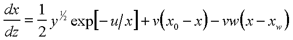
The non-dimensional equations describing the relationship between x and y are:

	(1)
	(2)

The following parameters apply:

u = 1.68
v = 3 x 10^-18

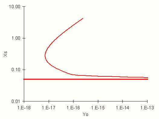
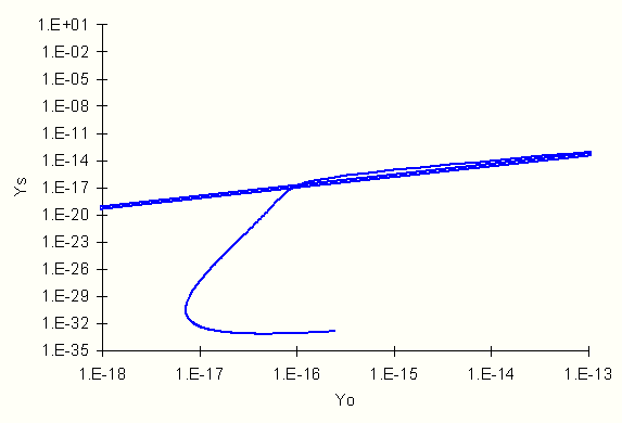
19. Prepare a graph of x_s versus y₀ for x₀ = 0.05 following the figure from Hoftyzer and Zwietering. Also prepare a graph of y_s versus y₀ for x₀ = 0.05. (Adiabatic Case)

For the steady state, adiabatic case equations (1) and (2) become:

	(3)
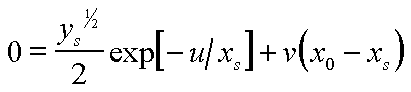	(4)

Now, solving (3) for y₀ and (4) for y_s yields:

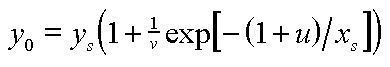	(5)
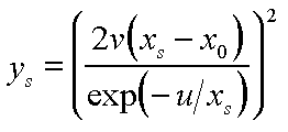	(6)

From these equations, the following graphs can be charted.

For x_s as a function of y₀ for x₀ = 0.05:

For y_s as a function of y₀ for x₀ = 0.05:

20. Solve for the steady state [non-dimensional] concentration and [non-dimensional] temperature when y₀ = 10^-16 and x_o = 0.05.

From the graphs in problem 19, it is evident there are 4 solutions to this problem: However, due to the huge gradient very close to xs=0.05, the solutions in that area could not be calculated. The values where xs > 0.06 are as follows:

(Using tolerances of 1 x 10^-8 to 1 x 10^-9 showed agreement to 6 significant figures)

21. Consider the reactor when the heat removal term just balances the heat generation term so that the temperature is constant. Prepare a graph of y_s versus y₀ for x_o = 0.05 under these conditions.

If dx/dz is zero, then x_s = x₀ for all z. Therefore equation (3) becomes:

(7)

When solved for y_s, equation (7) yields:

(8)

Which is a linear relationship with y₀. The following graph illustrates this:

Appendix, Calculations

The following Matlab functions were created for accomplishing this homework:

To solve Equation (5):

function yo=yo19(xs)
%
% Constants
%
u = 1.68 ;
v = 3.0e-18 ;
%
% Calculate yo
%
ys = ys19( xs ) ;
yo = ys * ( 1 + 1 / v * exp( - ( 1 + u ) / xs ) ) ;
end

To solve Equation (6)

function ys=ys19(xs)
%
% Constants
%
u = 1.68 ;
v = 3.0e-18 ;
xo = 0.05 ;
%
% Calculate ys
%
ys = ( 2 * v * ( xs - xo ) / exp( - u / xs ) ) ^ 2 ;
end

To help solve equation (5) for a given y₀ value.

function yo_diff = search20(xs)
yo_diff = 1 - yo19(xs)/(1e-16) ;
end

To solve equation (8):

function ys=ys21(yo)
%
% Constants
%
u = 1.68 ;
v = 3.0e-18 ;
xo = 0.05 ;
%
% Calculate ys
%
ys = v * yo / ( exp( - ( 1 + u ) / xo ) + v ) ;
end

Checking yo19 and ys19 by hand:

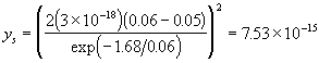
From the Matlab command line:

EDUª ys19( 0.06 )

ans =

      7.529974185646778e-015

EDUª yo19( 0.06 )

ans =

      7.630247500989692e-015

Which appear to agree.

Check search20 by hand:

From the Matlab command line:

EDUª search20( 0.06 )

ans =

      -7.530247500989694e+001

Which appears to agree as well.

Finally checking ys21:

(Which loses significant figures on my calculator, the exponential value is of the order of 1.1 x 10^-24 which is lost in the 3 x 10^-18 term-)

From the Matlab command line:

EDUª ys21( 1e-13 )

ans =

      9.999982433155688e-014

Which has more precision than my hand calculator.

The numbers for problem 19 were generated with the following script:

for i = 1:200 %also (1:400)

   xs( i ) = ( i + 2 ) / 1000 ; %also (i+20)/100

   ys( i ) = ys19( xs( i ) ) ;

   yo( i ) = yo19( xs( i ) ) ;

end

xs = xs'

ys = ys'

yo = yo'

plot(yo,xs)

and then copied into Excel for graphing. The numbers for Problem 20 were obtained by the following:

EDUª xs = fzero( 'search20', 0.048, 1e-8 )

xs =

   6.905973044876815e-002

EDUª xs = fzero( 'search20', 0.048, 1e-9 )

xs =

   6.905973044877588e-002

EDUª xs = fzero( 'search20', 2.0, 1e-8 )

xs =

   2.580376338595115e+000

EDUª xs = fzero( 'search20', 2.0, 1e-9 )

xs =

   2.580376338595115e+000

EDUª ys19( xs )

ans =

   8.475846061828390e-034

The following script was used to generate the data for problem 21.

for i = 1:180

yo( i ) = 10 ^ ( - i /10 ) ;

ys( i ) = ys21( yo( i ) ) ;

end

yo = yo'

ys = ys'

Return to Polymerization Page