Last updated: January
14, 2000
Note: These notes are preliminary and incomplete
and they are not guaranteed to be free of errors. Please let me know if
you find typos or other errors.
Combining the behavioral models for labor demand and labor supply together allows us to
deduce the equilibrium real wage and the equilibrium amount of employment.

In equilibrium, ND = NS which determines the equilibrium values of the real wage and
employment. It is implicitly assumed that in equilibrium everyone who wants a job has a
job. In this sense, the equilibrium value of employment is also called full employment.
When the labor market is in equilibrium, there is no tendency to move away from
equilibrium. That is, at the equilibrium values of w and N there are no
forces acting in the labor market to move the market away from the equilibrium values.
To understand equilibrium, it is helpful to see what happens when the labor market is
out of equilibrium. The figure below illustrates a situation where the current real wage
is higher than the equilibrium real wage.
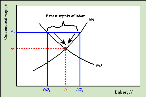
At w0 the supply of labor,
NS0 is greater than the demand for labor, ND0 , and so there is an
excess supply of labor in the labor market. Workers bid down the real wage until it falls
to the equilibrium value, w.
The above graph demonstrates that when the current wage is such that it is not equal to
the equilibrium real wage competitive market forces act to push the wage toward the
equilibrium wage. As the wage adjusts, labor demand and labor supply move closer to
equality.
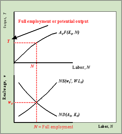
The labor market determines the equilibrium or full employment level of labor input to
the aggregate production function. Therefore, we define full employment output, Y*, in the following way:
Y* = A0F(K0,
N* )
where N* denotes the full employment
labor amount determined by equilibrium in the labor market.
Note: The textbook by Abel and Bernanke uses "bars" on top of
equilibrium values. Since I can't figure out how to put bars on top of letters in HTML, I
will denote an equilibrium value with a superscript "*" and the color red.
Full employment output is depicted in the graph below
Since the production function is linked with the labor market to determine full
employment (or potential) output, anything that shifts the production function (which
shifts labor demand) or the labor supply curve will affect potential output. To
illustrate, the graph below shows how potential output is affected by an increase in
productivity.
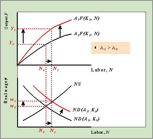
An Increase in productivity from A0
to A1 shifts up both the production function and labor demand (red curves). The
labor market then adjusts to a new equilibrium with a higher amount of employment and a
higher real wage. The increase in employment leads to a higher level of potential output.
Notice that output is higher both because the production function shifts up and because
employment increases.
