Last updated:
February 14, 2000
Note: These notes are preliminary and incomplete
and they are not guaranteed to be free of errors. Please let me know if
you find typos or other errors.
The aggregate demand for goods and services is determined at the intersection of the IS
and LM curves independent of the aggregate supply of goods and services (implicitly, when
deriving the AD curve it is assumed that whatever is demanded can be supplied by the
economy). The AD curve is a plot of the demand for goods as the general price level
varies. Hence, the AD curve gives all combinations of (P, Y) such that
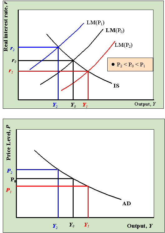
IS=LM. The derivation of the AD curve is illustrated below.

For a given price level, P0, the IS and LM curves intersect at the
point (r0, Yd0). This intersection
point is plotted in the graph below (as the big black dot). If the price level increases
to P1 then the LM curve shift up and left and the new equilibrium is
at the point (r1, Yd1). The higher real
interest rate has decreased the aggregate demand for goods. This new equilibrium is
represented as the big blue dot on the AD curve. Similarly, if the price level drops from P0
to P2 then the LM curve shifts down and right lowering the real
interest rate and increasing demand. This new equilibrium is given by the big red dot on
the AD curve.
The above graphs shows that the AD curve is a downward sloping function of the general
price level. This occurs because a decline in the general price level, P, (given
a fixed money supply, M) lowers the real interest rate, r, and
stimulates interest sensitive consumption and investment demand.
Rule 1: Anything
that shifts the IS curve up and to the right increases the aggregate demand for goods and
services and thus shifts the AD curve up and right.
Rule 2: Anything
that shifts the LM curve down and to the right increases the aggregate demand for goods
and services and thus shifts the AD curve up and right.
The main factors that influence demand are summarized in the
table below:
| Increase in Factor |
Shifts AD curve |
| Government spending, G |
Up and Right |
| Wealth, WL |
Up and Right |
| Lump-sum taxes, T |
Down and Left |
| Future marginal productivity of capital, MPKf |
Up and Right |
| Nominal Money Supply, M |
Up and Right |
| Expected inflation, pe |
Up and Right |
Assumptions Concerning the Long-run and Short-run
Long-run: Prices
and perfectly flexible and markets are in equilibrium. Firms are only willing to produce
output equal to full employment output.
Short-run: Prices
and wages are fixed and markets may be out of equilibrium (disequilibrium). Firms are
willing to "meet" the demand for goods and services by varying output and
employment.
The Classical Long-run Aggregate Supply Curve
The Classical long-run aggregate supply (ASLR) curve is derived from the
full employment (FE) curve. The ASLR curve is drawn in a graph with the
aggregate price level, P, on the vertical axis and output, Y, on the
horizontal axis. Recall, the aggregate supply of output is determined by the interaction
between the production function and the labor market as summarized by the FE line. In
labor market equilibrium, full employment output is Y*. Only changes in the
production function or changes in labor demand or labor supply will change Y*.
Since the production function and the labor market are not affected by changes in the
aggregate price level (it is assumed that any change in P is offset by changes in
nominal wages, W, so that the real wage, w = W/P,
stays constant) the aggregate supply curve is a vertical line in the graph with P
on the vertical axis and Y on the horizontal axis.
Factors the
Shift the Classical Long-run Aggregate Supply (ASLR) Curve |
Increase in Factor |
Shifts ASLR |
| Productivity, A |
Right |
| Capital stock, K |
Right |
| Wealth, WL |
Left |
| Labor force size, LF |
Right |
The Short-run (Keynesian) Aggregate
Supply Curve
Since in the short-run it is assumed that prices and wages are fixed and that firms are
able to "meet" demand the short-run aggregate supply curve is a horizontal line
in a plot with the general price level on the vertical axis and outout on the horizontal
axis.
The short-run aggregate supply (ASSR) curve will shift whenever prices
change in the economy. The ASSR shifts down when prices fall and it shifts up
when prices rise.
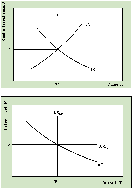
Recall, in general equilibrium (1) the labor market is in equilibrium; (2) the goods
market is in equilibrium; and (3) the asset market is in equilibrium. Using the IS/LM/FE
diagrams, general equilibrium occurs at the combination of (r, Y) where IS=LM=FE. General
equilibrium can also be illustrated using the AD/AS diagram: it is the combination of (P,
Y) such that ASLR = ASSR = AD. These relationships are depicted
below.


