Econ 301 Lecture 7

Reading: AB, chapter 7.
Last updated on February 19, 1997.

Topics

• Functions, properties and definitions of money
• The money supply
• Money demand
• Equilibrium in the money market

Functions, properties and definitions of money.

Functions and properties of money

• Medium of exchange
• Unit of account
• Store of value
• Low return (interest rate)
• Low risk
• High liquidity

Definitions of monetary aggregates

In this class, when we talk about the nominal money supply we will be referring to the monetary aggregate M1. Hereafter, the symbol "M" will denote M1.

The supply of money

The Fed and the supply of money

• The Federal Reserve Bank (Fed) ultimately controls the supply of money in the economy. The Fed is the central bank for the U.S. and is a quasi-private entity (technically owned by private banks) created by the Federal Reserve Act in 1913. There are twelve regional Federal Reserve Banks across the country and the leadership of the system is conducted by the Board of Governors of the Federal Reserve System (Federal Reserve Board ). The Board consists of seven governors, appointed by the President to staggered fourteen-year terms. The President appoints one Board member as chairman - currently Allen Greenspan - for a term of four years. It is important to keep in mind that the Fed operates independently of the federal government. Congress and the President does not have direct control over the operations of the Fed.
• The Fed primarily controls the supply of money (M1) in the economy through what are called open market operations. These are the purchase and sale of government bonds by the Fed. The Fed operates the printing presses for the creation of currency. The Fed also owns a substantial amount of U.S. government bonds. When the Fed wants to increase the supply of money it performs an open market purchase of government bonds. That is, the Fed buys (by printing money) outstanding government bonds from the public or new government bonds from the Treasury (to finance the current deficit). This operations injects new cash into the economy. Conversely, when the Fed wants to decease the amount of money in the economy it performs an open market sale of government bonds. Here, the Fed sells some of its holdings of government bonds to the public in exchange for cash. This operation takes cash out of the economy.

Money Demand

The demand for money

Consumption and saving decisions indirectly involve a decision about how much money to hold

• Individuals need money for transactions involving consumption goods and services. This is the transactions demand for money.
• Given income, what is not consumed is saved. Individuals must then decide how divide their savings into various kinds of assets: cash, savings accounts, government bonds, stocks etc. This is the asset allocation or portfolio problem. Since money pays very little interest (has a low return) the higher the interest rate on non-money assets the higher the opportunity cost of holding money.

Simplifying assumptions

Since the general asset allocation problem involves many different kinds of assets with different risk and return characteristics we simplify this decision by assuming that there are only two kinds of financial assets in the economy.

• Money assets - low return, high liquidity and low risk. i_m = nominal interest rate on money assets.
• Non-money assets (bonds) - higher return than on money assets and less liquidity. We assume that the risk associated with investing in bonds is not too high (think of government bonds as the generic non-money asset). Let i denote the nominal interest rate on non-money assets. Note that, by assumption, i > i_m. Also, recall that i = r +pi^e, where r denotes the real return on non-money assets and pi^e denotes expected inflation.

Model for money demand

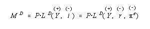
Our model for the demand for nominal money balances takes the following form:

where

• M^d = demand for nominal money balances (demand for M1)
• L^d = demand for liquidity function
• P = aggregate price level (CPI or GDP deflator)
• Y = real income (real GDP)
• I = nominal interest rate on non-money assets
• r = real interest rate on non-money assets
• pi^e = expected inflation

Remarks

• Nominal money demand is proportional to the price level. For example, if prices go up by 10% then individuals need 10% more money for transactions.
• As Y increases, desired consumption increases and so individuals need more money for the increased number of desired transactions.
• As the nominal interest rate on non-money assets, i, increases the opportunity cost of holding money increases and so the demand for nominal money balances decreases.
• Since i = r + ^e, we can decompose the effects on an increase in i into real interest rate increases (holding expected inflation fixed) and expected inflation increases (holding the real interest rate fixed).

The demand for real balances

Since the demand for nominal balances is proportional to the aggregate price level, we can divide both sides of the nominal money demand equation by P. This gives the liquidity demand function or the demand for real balances function:

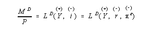
The left-hand-side of the above equation is the demand for nominal balances divided by the aggregate price level or the demand for real balances (the real purchasing power of money). The right-hand side is the liquidity demand function. The demand for real balances is decomposed into a transactions demand for money (captured by Y) and a portfolio demand for money (captured by i).

The real money demand function is graphed below:

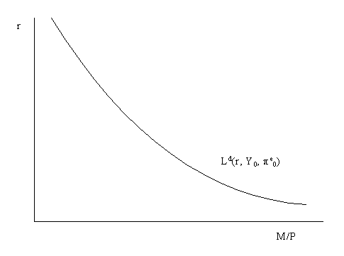
The demand for real balances is graphed as a function of the real interest rate holding income and expected inflation fixed. When the real interest rate is high the opportunity cost of holding money - keeping income and expected inflation fixed - is high so that real money demand is low. Conversely, when the real interest rate is low the opportunity cost of holding money is low so that money demand is high (due to the liquidity convenience of money over bonds). Whenever income or expected inflation change the real money demand curves shifts. For example, if Y increases the real money demand function shifts up and right; if expected inflation increases the real money demand function shifts down and left.

Equilibrium in the money market

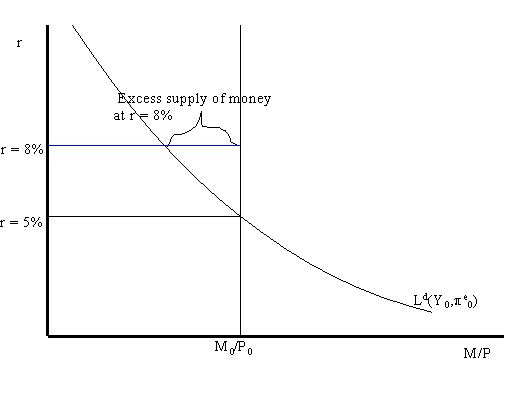
Real money demand and the real money supply as functions of the real interest rate are illustrated in the above graph. Real money demand is graphed holding fixed real income and expected inflation. The real money supply is equal to the nominal amount of M1, denoted M₀, divided by the fixed aggregate price level, P₀. It is assumed that the Fed does not alter the money supply based on the valued of the real interest rate. Therefore, the real money supply function is a vertical line in the graph with the real interest rate on the vertical axis and real money balances on the horizontal axis.

Notice that real money demand and real money supply intersect when the real interest rate is 5%. This is the value of the real interest that equates money demand with the money supply and establishes equilibrium in the money market. When the money market is in equilibrium there are no economic forces acting on the economy to alter the real interest rate.

If the real interest rate were 8% then the demand for real balances would be greater than the fixed supply of real balances (as illustrated above). In this case we say there is an excess supply of money in the money market. Practically, what this means is that individuals are holding more money than they would like given the high real interest rate. Accordingly, individuals will attempt to rebalance their portfilios; i.e. they will try to get rid of money by buying bonds (our generic non-money asset). In doing so the demand for bonds increases and so the price of bonds increases. Because bond prices are inversely related to the interest rate on bonds, the increased price of bonds lowers the real return on bonds (holding expected inflation fixed). Therefore, the excess supply of money at 8% (disequilibrium in the money market) leads to economic forces that act to lower the real interest rate. These forces cease to operate when the real interest falls to 5% where the demand for real balances is equal to the supply of real balances.

Comparative statics

Increase in the nominal money supply (M)

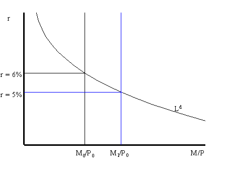
Consider the money market initially in equilibrium at r = 6% as illustrated in the above graph.. Suppose the Fed increases the nominal money supply by an open market purchase of government bonds. This increases the money supply from M₀ to M₁. Holding the price level fixed, this increases the supply of real balances from M₀/P₀ to M₁/P₀. If the real interest rate stays at 6% then the supply of real balances will be greater than the demand for real balances: there will be an excess supply of money in the money market. Consequently, individuals will try to get rid of the excess money by buying bonds which puts downward pressure on the real interest rate (holding expected inflation fixed). As r drops we move along the liquidity demand curve toward the new equilibrium at r = 5%.

Increase in the aggregate price level (P)

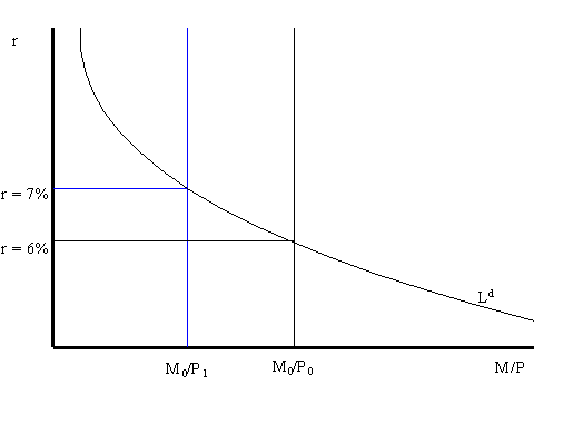
Consider the money market initially in equilibrium at r = 6% described in the graph below. Now suppose that the aggregate price level increases from P₀ to P₁. Holding the nominal money supply fixed, this reduces the supply of real balances from M₀/P₀ to M₀/P₁. If the real interest rate stays at 6% the supply of real balances will be less than the demand for real balances: there will be an excess demand for money. The excess demand for money will prompt individuals to sell bonds (demand for bonds falls) and so the real interest rate on bonds will rise. As r rises, we move up along the liquidity demand curve toward the new equilibrium at r = 7%.

Increase in current income (Y)

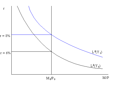
Consider the money market in equilibrium at r = 6% as illustrated above. Suppose that current income (Y), which is the same as current output (GDP),. Increases from Y₀ to Y₁. This increases the transactions demand for money as so the real money demand curve shifts up and to the right. If the real interest rate stays at 6% there will be an excess demand for money which puts upward pressure on the real interest rate. As r increases, we move along the money demand curve up towad the new equilibrium at r = 8%.