Modeling consumption and saving

Reading: AB, chapter 4, section 1.

Aggregate demand, the desired amount of aggregate expenditure, can be discussed in terms of desired consumption expenditure, C^d, and desired investment, I^d, or in terms of desired national saving, S^d, and desired investment. The reason is that we define desired national saving as: S^d = Y - C^d - G₀.

Behavioral model for national saving

By definition, saving is what is left over from current income after we have decided how much to consume. Decisions about consumption and saving involve decision about how much to consume today and how much to consume in the future. After all, the reason we save is so that we have wealth in the future, when we are no longer working, so that we can maintain consumption. Accordingly, any reasonable model for consumption and saving must take into consideration factors that influence our consumption today and our consumption in the future. Our model for national saving (private saving plus public saving) is of the form:

where

r = real interest rate

Y = real GDP (income)

FY^e = expected future income

WL = wealth

G = government spending.

Remarks

• As r increases the return to saving increases so desired saving increases and consumption decreases (holding income fixed). Also, a higher real interest reduced interest sensitive consumption (big ticket items like cars, refrigerators etc).
• As Y increases both desired saving and consumption increase. Generally, individuals consume more when their current income rises. A general rule of thumb is that consumption increases by about 90 cents for every dollar increase in income. Therefore, saving increases by about 10 cents for every dollar increase in income.
• As FY^e increases, while current income stays fixed, consumption tends to rise so that saving falls.
• Increases in G leads to decreases in savings since S^d = Y - C^d - G₀.

Income and substitution effects

Increases in the real interest rate affect desired saving in two different ways:

• Substitution effect: As r increases, the return to saving increases and this leads individuals to substitute current consumption for future consumption so that saving increases.
• Income effect: As r increases, for a target saver (someone who is saving for a particular target like a house), the target can be achieved with a smaller pool of saving. If individuals prefer more current consumption to future consumption than an increase in r will lead to less saving today and more consumption. For example, to have $10,000 in one year when r = 5% requires one to save $9,524 = $10,000/(1.05). If r increases to 10% then one only has to save $9,091 = $10,000/(1.10). Consumption can go up by almost $500 and the desired target can still be achieved.

Graphical representation of desired saving

The relationship between desired national saving and the real interest holding fixed Y, FY^e, WL and G is called the savings curve and is illustrated below:

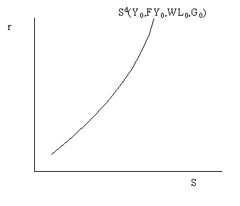
The savings curve is steep because the substitution effect is empirically very weak: it takes a very large increase in the real interest rate to induce individuals to save more. The savings curve shifts out and to the right (savings increases) when either Y, FY^e or WL increases. Conversely, the savings curve shifts up and left (savings decreases) whenever G increases.