Econ 301 Lecture 5

Reading: AB, chapter 3; chapter 8, section 5 (skim - advanced section)
Last updated on July 18, 1996.

Contents

• Unemployment definitions and statistics
• Introduction to the demand side of the economy
• Modeling consumption and saving
• Modeling investment

Unemployment definitions and statistics

Types of Unemployment

• Frictional Unemployment: unemployment caused by workers searching for jobs and firms searching for workers.
• Structural Unemployment: long-term chronic unemployment that exists when the economy is not in a recession. The main causes of structural unemployment are: (1) the number of low skilled workers exceeds the number of low skilled jobs (dual labor market idea); (2) some sectors of the economy are contracting while others are expanding and the contracting industries create unemployment.
• Natural Rate of Unemployment: unemployment rate consistent with full employment = frictional rate + structural rate = u*. Currently the natural rate is estimated to be somewhere between 5.5% and 6.5%. However, it is not estimated very precisely. (Note: equilibrium values are denoted with a superscript "*" instead of an overbar since I can't get overbars to print in HTML.)
• Cyclical Unemployment: actual rate of unemployment - natural rate of unemployment = u - u*. The cyclical rate of unemployment is the unemployment created by recessions and booms. During recessions, u - u* > 0; during booms, u - u* < 0.
• Actual Unemployment Rate: natural rate + cyclical rate = u = u* + (u - u*).
• NAIRU: non-accelerating inflation rate of unemployment = rate of inflation consistent with stable prices/inflation = natural rate of unemployment. The NAIRU and the natural rate are the same thing. As we shall see, the natural rate of unemployment (NAIRU) is the rate of unemployment that exists when inflation is neither increasing nor decreasing. When the economy is booming, cyclical unemployment is positive and inflation tends to accelerate; when the economy is in recession, cyclical unemployment is negative and inflation tends to decelerate.

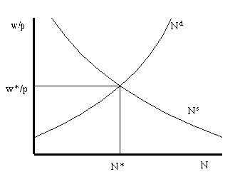
Graphical illustration of u*

The natural rate of unemployment, u*, is the unemployment rate that occurs when the labor market is in equilibrium; i.e. when employment is N*.

Unemployment Statistics

• Labor force (LF): number of employed individuals (E) + number of unemployed individuals seeking work (U).
• Not in the labor force (NLF): those individuals neither employed nor unemployed and not seeking work.
• Adult population: LF + NLF.
• Unemployment rate: u = U/(E + U). Note that the unemployment rate changes whenever U or E changes.

[insert pie chart of unemployment statistics here]

Counter Intuitive Facts About Unemployment

• Most spells of unemployment (i.e., time spend unemployed) are short - about 2 months
• Most people who are unemployed on a given date are experiencing long unemployment spells (i.e., have been unemployed for a long time - about 1 year).

Introduction to the demand side of the economy

Overview

Our discussion so far of the labor market and the production function represents the supply-side of the economy independent of the overall level of aggregate demand. Changes in factors that affect labor demand (N^d), labor supply (N^s) and the production function (F) change the potential supply, Y*, of the economy independent of demand. (Note: variables with supercript "*" are equilibrium values.)

The demand-side of the economy focuses on the aggregate demand for goods and services independent of potential supply. To simplify our analysis, we assume that there is no foreign sector to the economy. Then aggregate demand for goods and services, using the expenditure approach, is defined as: Y^d = C^d + I^d + G₀, where C^d = demand for consumption goods, I^d = demand for investment goods and G₀ = exogenous government spending on goods and services. Here, NX = 0 since there is no foreign sector. Modeling the aggregate demand for goods and services thus requires modeling the demand for consumption goods and the demand for investment goods. However, since desired national saving is defined as S^d = Y^d - C^d - G₀ we may also focus on modeling saving behavior instead of consumption behavior.

Modeling consumption and saving

Aggregate demand, the desired amount of aggregate expenditure, can be discussed in terms of desired consumption expenditure, C^d, and desired investment, I^d, or in terms of desired national saving, S^d, and desired investment. The reason is that we define desired national saving as: S^d = Y - C^d - G₀.

Behavioral model for national saving

By definition, saving is what is left over from current income after we have decided how much to consume. Decisions about consumption and saving involve decision about how much to consume today and how much to consume in the future. After all, the reason we save is so that we have wealth in the future, when we are no longer working, so that we can maintain consumption. Accordingly, any reasonable model for consumption and saving must take into consideration factors that influence our consumption today and our consumption in the future. Our model for national saving (private saving plus public saving) is of the form:

where

• r = real interest rate
• Y = real GDP (income)
• Y^e = expected future income
• WL = wealth
• G = government spending.

Remarks

• As r increases the return to saving increases so desired saving increases and consumption decreases (holding income fixed). Also, a higher real interest reduced interest sensitive consumption (big ticket items like cars, refrigerators etc).
• As Y increases both desired saving and consumption increase. Generally, individuals consume more when their current income rises. A general rule of thumb is that consumption increases by about 90 cents for every dollar increase in income. Therefore, saving increases by about 10 cents for every dollar increase in income.
• As FY^e increases, while current income stays fixed, consumption tends to rise so that saving falls.
• Increases in G leads to decreases in savings since S^d = Y - C^d - G₀.

Income and substitution effects

Increases in the real interest rate affect desired saving in two different ways:

• Substitution effect: As r increases, the return to saving increases and this leads individuals to substitute current consumption for future consumption so that saving increases.
• Income effect: As r increases, for a target saver (someone who is saving for a particular target like a house), the target can be achieved with a smaller pool of saving. If individuals prefer more current consumption to future consumption than an increase in r will lead to less saving today and more consumption. For example, to have $10,000 in one year when r = 5% requires one to save $9,524 = $10,000/(1.05). If r increases to 10% then one only has to save $9,091 = $10,000/(1.10). Consumption can go up by almost $500 and the desired target can still be achieved.

Graphical representation of desired saving

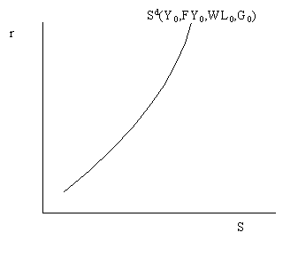
The relationship between desired national saving and the real interest holding fixed Y, FY^e, WL and G is called the savings curve and is illustrated below:

The savings curve is steep because the substitution effect is empirically very weak: it takes a very large increase in the real interest rate to induce individuals to save more. The savings curve shifts out and to the right (savings increases) when either Y, FY^e or WL increases. Conversely, the savings curve shifts up and left (savings decreases) whenever G increases.

Modeling Investment

Determinants of Investment Behavior

Recall, investment expenditure refers to the purchase of physical capital for the purpose of increasing future output. In the National Income and Product Accounts, investment is broken into business fixed investment (investment in equipment and structures) and inventory investment (purchase of unsold production). In this section we only model the demand for business fixed investment.

Some definitions

• I(t) = gross investment during year t (flow variable).
• K(t) = capital stock at the beginning of year t (stock variable).
• K(t+1) = capital stock at the beginning of year t+1.
• d = rate of depreciation of the capital stock (e.g. d = 10%).
• Net investment = gross investment - depreciation = K(t+1)-K(t) = I(t) - d*K(t), where K(t+1)-K(t) is the net change in the capital stock from year t to year t+1; I(t) is gross investment; and d*K(t) is the amount by which the capital stock in year t depreciates or wears out.

Example

Let K(1995) = $100 billion, K(1996) = $110 billion and d = 10%. Net investment is equal to K(1996)-K(1995) = $10 billion. The depreciation of the capital stock over 1995 is 0.10*$100 billion = $10 billion. Then gross investment over 1995 is: I(1995) = net investment + depreciation = $10 billion + $10 billion = $20 billion.

Behavioral Model for Gross Investment

Firms invest in physical capital when they want to expand the scope of operation and production. Firms decide to take on investment projects when the expected benefits of investment (returns to investment) outweigh the expected costs. This decision is called the capital budgeting decision and it is discussed in great detail in courses in financial economics. For our purposes, we simply need to recognize that firms invest when the expected net benefits from investment projects is positive. The textbook goes into a detailed discussion of how firms weigh the costs and benefits of an investment project and I will just summarize the main results here:

• The expected return from an investment project is measured by the expected future marginal product of capital (FMPK) that is generated by the investment. Whenever FMPK is high, desired investment tends to increase.
• Most firms need to borrow in order to finance large investment projects. The expected real interest rate, r, captures this borrowing cost to firms. When r is high, the cost of borrowing is high and desired investment tends to decrease.

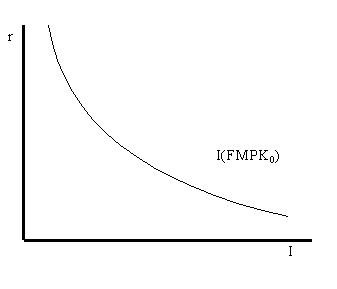
Our behavioral model for investment is given by

and is given graphically by

As the above graphs shows, for a fixed level of FMPK desired investment is low when the real interest rate, r, is high and desired investment is high when the real interest rate is low. The investment graph will shift up and to the right when FMPK increases and it will shift down and to the left when FMPK decreases.