Here are two approaches for fitting multiple modes to univariate data: using histogram data and probability density functions.

            Histogram data

The method of Macdonald & Green (1988) analyses histogram data which is the most frequent representation for plant population data.    It finds the best fit for component distributions using chi-squared approximation to the likelihood ratio test using grouped data (Macdonald & Pitcher 1979; Macdonald 1987).   Grouping data simplifies calculation of maximum likelihood estimates but Macdonald & Green warn against histogram groups with zero data or small numbers.   The mixdist package, an implementation in R of the MIX package (Macdonald & Green 1988) can fit other component distribution types than just the normal including lognormal and gamma.   mixdist calculates parameter values and their standard errors for each distribution in the mixture and chi-square for the fit between empirical histogram and the histogram calculated from the sum of the mixture distributions.   mixdist can be used in exploratory analysis of numbers and types of component distributions that give effective fits.

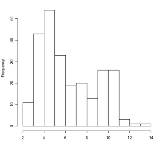
Using the R programming language you can investigate fitting a bimodal distribution to histogram data using mixdist.   You must first install the package and then load it.   The data used as an example is of plant height and plant weight of 250 dwarf marigold plants 42 days after sowing closely together.   A histogram of the height data (shown at right) can be obtained by the R command: > hist(Ht.data) The scale of the x axis is centimeters and frequency is number of plants.  The function hist calculates the number of bins into which values are sorted. This can be regulated using the breaks parameter of that function.

In order to use mixdist the data for a histogram must be presented for the bins, sequentially and in increasing ordinate value, with the upper division value of a binfollowed by the number of values in that bin.   The last bin must have with an upper division of infinity.   On the left is a function that divides data into a specified number of bins and outputs the data in the form required by mixdist using the as.mixdata function.

function(ddata, bins, resolution){ # # Function to create a histogram of non-zero data for use in # the mix.dist program # # !! REQUIRES THAT THE PACKAGE "mixdist" IS ATTACHED !! # # Call: mix.dist.hist <- make.mix.data(ddata, bars, resolution) # # ddata: array of single value, non-zero, variables # bins: Number of groups in the histogram # # data.out: A two dimensional array of histogram-type grouped data # with first column the upper bound value of the interval and # second column the number of values in the interval # data.out <- matrix(0, bins, 2) nvals <- length(ddata) # # Create histogram intervals # max.ddata <- max(ddata) min.ddata <- min(ddata) offset <- (max.ddata - min.ddata)/resolution a <- min.ddata inter <- ((offset + max.ddata) - (min.ddata-offset))/bins for (i in 1:bins){    a <- a + inter data.out[i, 1] <- a } # # Partition the data into bins # for (i in 1:nvals){    k <- 1    calc.x <- ddata[i] - min.ddata    while (calc.x > inter){       calc.x <- calc.x - inter       k <- k + 1    }    data.out[k, 2] <- data.out[k, 2] +1 } data.out <- as.mixdata(as.data.frame(data.out)) data.out }

Th following code takes the output from the above function, mix.dist.hist, and provides a summary of the fit obtained. The output from plot(fitdummy1) is shown on the right. > fitdummy1 <-mix(mix.dist.hist, mixparam(mu=c(10, 15), sigma=c(1,1)), "norm") > summary(fitdummy1) Parameters:    pi      mu    sigma 1 0.6973 4.790   1.333 2 0.3027 9.785   1.102 Standard Errors:    pi.se    mu.se    sigma.se 1 0.0424    0.1558   0.1340 2 0.0424    0.2685   0.2230 Analysis of Variance Table           Df   Chisq   Pr(>Chisq) Residuals 7   23.593   0.001343 ** --- Signif. codes: 0 ‘***’ 0.001 ‘**’ 0.01 ‘*’ 0.05 ‘.’ 0.1 ‘ ’ 1 > plot(fitdummy1)

The individual normal distributions are represented by dashed lines and their sum by the solid line. Estimates of the mean values are indicated by arrow head marks on the x axis

The goodness-of-fit is the chi-squared approximation to the likelihood ratio statistic (see Users Guide for MIX). It is possible to fit different numbers of mixtures. An obvious case to try is that of a single distribution using the instruction: > fitdummy1 <-mix(mix.dist.hist, mixparam(mu=c(8), sigma=c(2)), "norm") This has more degrees of freedom (because fewer parameters are being estimated) and actually gives a lower p value than the fit for two modes. > fitdummy1 <-mix(mix.dist.hist, mixparam(mu=c(10, 15), sigma=c(1,1)), "norm") > summary(fitdummy1) Parameters:    pi      mu    sigma 1   1     6.263   2.694 Standard Errors:    pi.se    mu.se    sigma.se 1     NA    0.1722   0.1272 Analysis of Variance Table           Df   Chisq   Pr(>Chisq) Residuals 10   100.11   2.2e-16 *** --- Signif. codes: 0 ‘***’ 0.001 ‘**’ 0.01 ‘*’ 0.05 ‘.’ 0.1 ‘ ’ 1 > plot(fitdummy1)

Although the significance of the fit is greater than that for two modes the residuals between fitted line and histogram have a marked pattern with four central bins all being less than the fitted line while, on either side, there are bins with greater values than the fitted line.

             Probability density functions

An alternative approach to fitting mixture distributions is based on probability density functions rather than histograms.   Maximum likelihood estimates of parameters are found using an expectation-maximization (EM) algorithm (Leisch 2004) as implemented in the R package flexmix (Leisch and Gruen 2010).   Models with different numbers of mixture components can be compared using the Akaike and Bayesian Information criteria.

To use flexmix the data must be in the form of a data frame.  The instruction: ht.data <- as.data.frame(Ht.data) will produce the data frame ht.data with the column of height data labelled as Ht.data.   The following instructions calculate first a mixture of two normals (with k=2) and provide a log likelihood estimate and AIC and BIC values and then a sinle normal distribution (k=1) with its AIC and BIC values. > fl <- flexmix(Ht.data~1, data = ht.data, k=2) > summary(fl) Call: flexmix(formula = Ht.data ~ 1, data = ht.data, k = 2)         prior   size   post>0   ratio Comp.1   0.371    91    247     0.368 Comp.2   0.629   159    201     0.791 'log Lik.' -545.6951 (df=5) AIC: 1101.390   BIC: 1118.997 > parameters(fl)                    Comp.1       Comp.2 coef.(Intercept) 9.279662     4.564806 sigma            1.497320     1.079630    > fl <- flexmix(Ht.data~1, data = ht.data, k=1) > summary(fl) Call: flexmix(formula = Ht.data ~ 1, data = ht.data, k = 1)           prior size     post>0 ratio Comp.1     1     250      250      1 'log Lik.' -593.3792 (df=2) AIC: 1190.758     BIC: 1197.801 > parameters(fl)                     Comp.1 coef.(Intercept)   6.314800 sigma              2.602775    With this method of calculation the mixture of two distributions is a better fit (having lower AIC and BIC values) than a single distribution.  Everitt and Hothorn (2006) give R code for plotting the estimated distributions relative to a histogram of data.

Return to "Methods and Software for Analysis of Population Structure"

References

Everitt, B.S. & Hothorn, T. (2006) A Handbook of Statistical Analyses Using R. Chapman & Hall, Boca Rotan.
Leisch, F. (2004) A general framework for finite mixture modesl and latent class regression in R. Journal of Statistical Software, 11. http://www.jstatsoft.org/v11/i08/
Leisch, F., Gruen, B. (2010) flexmix: Flexible mixture modelling. The Comprehensive R Archive Network, http://cran.r-project.org/index.html.
Macdonald, P.D.M. (1987) Analysis of length-frequency distributions. Age and Growth of Fish (eds R.C. Summerfelt & G.E. Hall), pp. 371-384. Iowa State University Press, Ames Iowa.
Macdonald, P.D.M. & Green, P.E.J. (1988) User’s Guide to Program MIX: An interactive Program for Fitting Mixtures of Distributions. Ichthus Data Systems, Hamilton, Ontario.
Macdonald, P.D.M. & Pitcher, T.J. (1979) Age-groups from size-frequency data: a versatile and efficient method of analysing distribution mixtures. Journal of the Fisheries Research Board of Canada, 36, 987-1001.