Notes on Mapping, Projections and Data AnalysisThese are some notes regarding possible pitfalls in projecting (lat,lon) onto (x,y) in geophysical or oceanographic data analysis. The issues discussed here may be obvious; I've always had them in the back of my mind as nagging suspicions; but here they are explicitly discussed. Matlab scripts for both a numerical solution, and the analytical solution, for the Chamberlin Trimetric Projection are given. The analytical (?) or numerical (?) solution, which is for the sphere only, is transcoded from QBASIC (!) code from John P. Snyder's suite of mapping programs. The QBASIC routine is also given. Table of Contents
IntroductionI recently ran into an issue in data analysis and mapping projection that I should have known about, but perhaps had forgotten. When data are collected in the field, they are usually obtained at some set of (lat,lon). Unless one is doing subsequent analysis of these data in spherical coordinates, one often has to project the locations onto a suitable cartesian grid (X,Y). The selection of that projection can be important because, with a poor projection, subsequent data analysis can be a little erroneous. It also seems to me that oftentimes after an expensive and lengthy analysis of expensive data, many people will plot their fabulous results up in (lon,lat) on a cartesian grid using no projection at all. While not erroneous per se, the results so displayed are rather badly distorted in shape from reality. I am beginning to wonder if constant exposure to misshapen results, say, starts to affect physical intuition. I therefore advocate a change in culture so that geophysical scientists will be more careful about how things are displayed in maps. In both of these points, I mean to suggest that how things are projected or displayed can have greater consequences than just esthetics. Cartography is often seen as just an esthetic endeavor - how to make a map just look a little better - but there may be substantive consequences to a lazy attitude toward the issue.
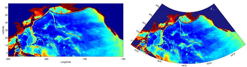
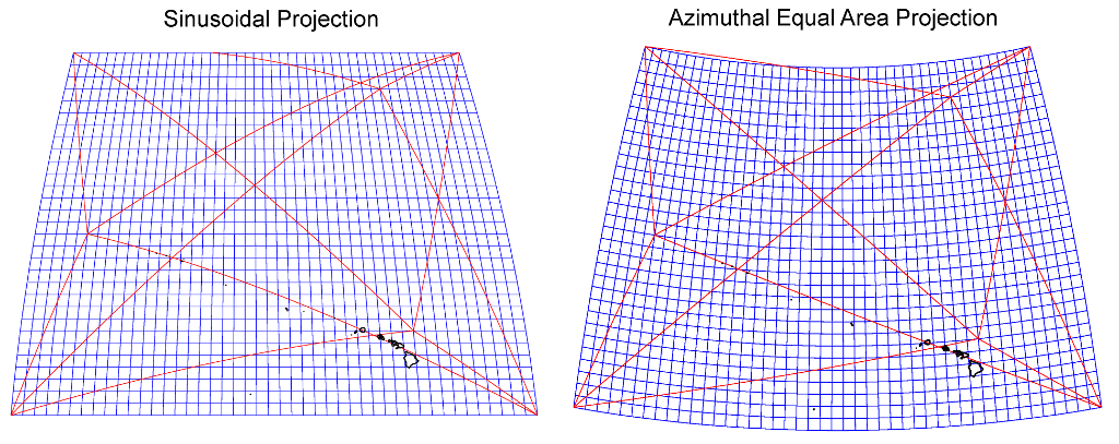
The same data (bathymetry of the North Pacific) shown lazily with no projection (left), and with the Lambert Conformal Conic Projection (right). The projection is made using the M_Map package for matlab; see Links. Which figure describes the physical world better? An Extreme ExampleA post-doc goes out in the field and deploys a set of instruments in a circular pattern over a large area. After a while, all the data are collected and taken back to the laboratory. The data analyst then projects the locations of the instruments using a projection with the property that the Y distances are grossly distorted relative to the X distances. Plotted in X-Y, the array looks like a flattened ellipse. The analysis procedes, a wavenumber spectrum is calculated. The scientist looking at the results concludes with the amazing "discovery" that the wavenumber spectrum is non-isotropic, and soon publishes the paper in Nature about the non-isotropic nature of the observed variability. Years pass, and the scientist, now a Senior Professor, is one day approached by his/her graduate student who, using a more accurate projection, suggests that the spectrum is isotropic. The Senior Professor tells the student that he/she is all wet, it is "well-known" that the spectrum is non-isotropic, "that's been published", and to go away and redo the analysis. The Senior Professor then complains to his/her peers about how hard it is to find good graduate students these days. The student reacts with two possibilities: (a) discouraged and thinking he/she is not up to par in figuring things out, quits and goes to work for Microsoft, or (b) the student concludes that the Senior Professor is an arrogant... well, never mind. A key point here is that the substantive problems arise when the analysis requires a parameter in relation to position. In this example, it is wavenumber and the physical property is phase = K*X. With an assumed wavenumber and a poorly chosen projection, the phases in the projected space are distorted relative to phases in the real world. Comparison of Sinusoid and Azimuthal Equal Area ProjectionsA comparison of two projections illustrates the problem. The figures below compares the Sinusoidal Projection against the Azimuthal Equal Area Projection. The Sinusoidal Projection is just the commonly used x=R*(λ - λ0)*cos(φ), y=R*(φ- φ0), where λ is longitude and φ is latitude (this simple projection was the source of my recent troubles). The area plotted is about 4000 km × 3000 km just north of Hawaii. Plotted on these figures are geodesics originating from three points. The Sinusoidal Projection suffers from two basic problems: (1) the geodesics are not straight lines, and (2) the distances across the projected area are not correct (range ≠ √ (ΔX2 + ΔY2) ). Both of these properties are generally desirable when an analysis is concerned with wave properties. As one colleague pointed out, waves travel along geodesics - if one's geodesics are not straight, one sees some strangely propagating waves... It should be noted that no one projection is suitable for all applications - this discussion is to suggest that any analysis should employ a projection that is selected to reduce errors in subsequent analysis. Projections have different properties of shape, distance, direction, etc. and no one projection is error free. Whatever projection is selected should lend errors that are at least acceptable.
Projection of (lat,lon) to (x,y) using m_mapCode to project from (lat,lon) to (x,y) using the m_map package is simply:
m_proj('lambert','long',[-200 -110],'lat',[15 60]); % Defines the projection to be used, Lambert Conformal Conic Projection. The m_proj routine includes a large number of possible projections, perhaps called with different parameters. See the M_Map web page for details; see Links. The reference "An Album of Map Projections" gives the formulas for a large number of projections; see Links. One can also employ the Generic Mapping Tools (GMT) package for projections; see Links.
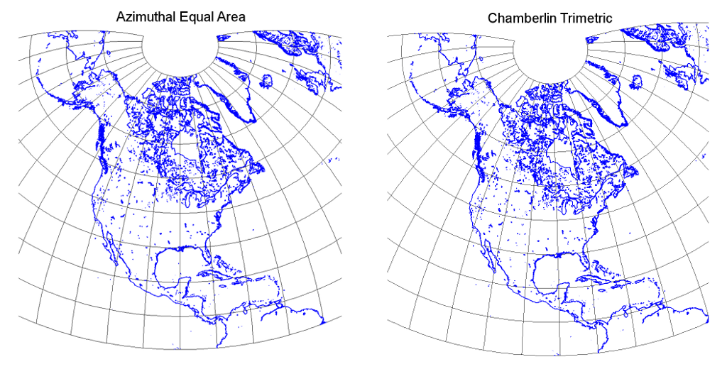
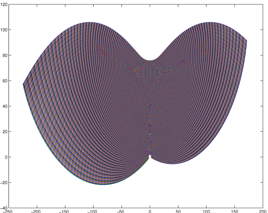
The Chamberlin Trimetric ProjectionIn snooping through the subject of cartography, I ran across several mentions of a projection known as the "Chamberlin Trimetric Projection". This projection maps (lat,lon) to points that are scaled by (almost) accurate distance from three preselected locations. The projection originates from National Geographic Society and is most often used by them for certain maps. The equidistance property seemed to be one that had the admirable qualities I was looking for, but, alas, no formulas for the projection are readily available. There are hints that the formulas are formidable. The projection was originally done graphically. From the description of the projection, however, it seemed easy enough to code in matlab by brute force. The idea is to calculate the positions (X,Y) ↔ (lat,lon) on a grid as tables, and subsequently use interpolation for the projection of any arbitrary point. For all the labor, the result of the Chamberlin Trimetric Projection was just slightly different than the Azimuthal Equal Area Projection, as seen below. Over a large area there may be differences, but over smaller regions the differences seemed negligible for my analysis. The Chamberlin Projection is usually used to map continental sized area or smaller; it is not suitable for the entire globe. The projection is a low-error compromise used because it has a nice balance of distortion - length, area, direction, etc. it is inherently an approximate three-point equidistant projection. Since no implementation of this projection is readily available, I include it here. It requires the m_idist routine of the M_Map package (link below) and through m_idist by default the projection employs the WGS'84 elipsoidal earth. The calls to m_idist can be modified to use the spherical earth or another ellipsoid. With the sets of matrices (X,Y) ↔ (lat,lon), the inverse is well defined. That is, given any arbitrary point (x,y), the matrices (X,Y) ↔ (lat,lon) defined on the grid can be used to obtain the latitude and longitude of it by interpolation. There are two main issues with the implementation of this projection: (1) Away from the segments of the triangle of the defining three points, no point can have an accurate distance from three points. The circular arcs of distance from the three points do not cross at a single point. The projected point is found by calculating the centroid of the three almost co-located points where the arcs cross. The projection is therefore not mathematically precise. The errors introduced by this brute-force implementation are likely minimal compared to the errors inherent in any projection, however. (2) Near the lines connecting any two points of the defining three points, the points of intersection of the arcs become close together such that the centroid point to be selected becomes ambiguous - there are two "best" points close together and it is not immediately apparent which one is correct. The routine here is designed to select those centroid points that lie on the regular grid (hopefully). This whole issue arises because three points are used to calculate the distances; the issue becomes moot if four points are employed. In any case, a routine that can accept an arbitrary point for projection is not possible with this approach. The grid is calculated so that points that do not fit the pattern of the grid can be found and corrected. For individual points, there is no way of assuring that the projected points are not in error. Hence, the projection of individual points are best obtained by interpolation using the regular grid. That said, it certainly appears as if the numerical approach results in a projection with a 2nd derivative that has a very well behaved pattern. The 2nd derivative, shown below, seems to me to be a critical test of smoothness and grid regularity. The sorts of irregularities noted in the Christensen reference below are not apparent.
The three source points for this map in the Chamberlin Projection, as selected by the National Geographic Society, are: (55° N, 150° W), (55° N, 35° W), and (10° N, 92°30' W). These were calculated to match the example in "An Album of Map Projections", p. 171, see Links. The Azimuthal Equal Area projection was calculated using M_Map; see Links.
This figure shows the 2nd derivative of the projection. The regular grid over the large domain of the figures above was calculated at 1/4 degree interval, or roughly 25 km X 25 km. This figure was plotted as "plot(diff(diff(X)),diff(diff(Y))); hold on; plot(diff(diff(X))',diff(diff(Y))'). The great regularity and smoothness of the grid shown here demonstrates that the grid of X,Y is quite well behaved. Matlab source code:chamberlin.m: The Chamberlin Trimetric Projection - numerical solution. This routine returns grids of (X,Y) associated with (lat,lon). (N.B. As of January 2010 this routine appears to be bug free, but it is not well tested.) Requires the routine m_idist from the M_Map package; see Links. chamberlin_test.m: An example routine that invokes the numerical solution for the Chamberlin trimetric projection. chamberlin_p.m: The Chamberlin Trimetric Projection - the analytic solution, on a sphere. This routine was transcoded from the QBASIC code snipped listed below. (N.B. As of January 2010 this routine appears to be bug free, but it is not well tested.) The routine here is only for a sphere (no ellipsoid solution) and an analytic inverse for it does not exist, to my knowledge. One could determine the inverse by interpolation using a grid, however. ADDED LATER: Now that I think about it, I think the code here may be just a more clever way of implementing the projection numerically, i.e., solving for the intersection points of the circular arcs. At the end of the routine, you'll see that three points are averaged, much like the routine I developed. There is no "direct" solution for the projection points, as it were. It does avoid the problem of having to project a grid and then do interpolation, however.
QBASIC source code:
The code below, apparently the analytic forumla for the Chamberlin
Trimetric Projection, is extracted from a zip file of BASIC source code
by John P. Snyder. It is from one file of many from Snyder's personal
suite of mapping programs. I extracted it from the full zip file
available here: http://www.galleryofmapprojections.com/snyder/snyder_full.zip CHAMBERLIN.QBASIC: Original QBASIC code due to John P. Snyder - Released to Public Domain by him.
References (found after the fact):Christensen, Albert H.J., The Chamberlin Trimetric Projection, Cartography and Geographic Information Science, Volume 19, Number 2, April 1992 , pp. 88-100(13) Abstract: A computer solution to the Chamberlin Trimetric projection is presented with a numerical method that circumvents the need for closed formulas to analyze distortions. The existence and consequence of singularities in the computer algorithms are discussed in detail, with suggestions to minimize their adverse effect. Linear, area, and angular distortions are estimated for the Chamberlin projection, and compared with values analytically computed for the Transverse Mercator and Albers Equal-Area Conic projections. In addition, distance distortions for the three projections are computed, listed, and compared. The author concludes that the Chamberlin projection is an excellent compromise between the other two, provided the discontinuities are resolved. Bretterbauer, Kurt (1989). "Die trimetrische Projektion von W. Chamberlin". 39. Kartographische Nachrichten. pp. 51–55. : Translation to English by Hugh Casement: CHAMBERL.DOC
Links
-- BrianDushaw - 18 Dec 2009 Copyright © 2008-2015 by the contributing authors. All material on this collaboration platform is the property of the contributing authors. |