QSCI 482 Prof. Conquest TAs Kennedy, Malinick, Norman

HW 7--DUE FRIDAY, DECEMBER 6, 2002

1. Scientists conducted a survey of stream segments in western

Washington to assess the effect of three different levels of commercial

timber harvest (none, moderate, intensive) on instream salmon spawning

habitat. One of the responses measured on each stream segment (the

sampling unit) was the percent of stream area comprised of pools. (Pools

are related to needed habitat for salmon spawning.) Data and

the summary statistics are as follows:

NONE: 43, 73, 36, 46, 42. n = 5, xbar=48.00, s^2=208.50.

MODERATE: 39, 62, 20, 44. n = 4, xbar=41.25, s^2=298.25

INTENSIVE: 37, 14, 21, 30, 07. n = 5, xbar=21.80, s^2=144.7.

1a. At the .05 level of significance [and assuming normality and equal

variances], test to see whether the three levels of timber harvest yield

the same mean pool fraction of stream area. Include the complete analysis

of variance (ANOVA) table. You may do this either by hand (it is indeed

do-able by hand) or by using statistical software like SPSS. NOTE: in

writing up your "conclusions" statement, AVOID the words "accept",

"reject", and "hypothesis"; rather, express conclusions in terms of the

original research question.

MSTr = 915.65, df=2; MSE=209.78, df=11

F = 915.62/209.78 = 4.365

F_0.05(1),2,11 = 3.98; Since 4.365>3.98 we reject the F-test (p=0.0402). Salmon spawning habitat (represented by % pools) is significantly different among levels of timber harvest.

1b. Are the three levels of timber harvest a "fixed effects" model or a

"random effects" model? Explain your answer.

The levels of timber harvest are fixed effects; if we were to repeat the study we would use the same three harvest levels.

1c. If we were to use a sample size of n=6 for each group (total sample

size = 18), how far apart would the largest and smallest population

means have to be in order to reject the null hypothesis with 90% power

and level of significance = .05?

For n = 6, df would be 18-3=15. Φ~2.3

δ = sqrt(2*3*2.3²*209.78/6) = 33.21

The largest and smallest means would need to be 33.21 percent pools apart to reject with 90% power and 0.05 significance.

1d. Now, at the alpha = 5 percent level of significance, do a parametric

(normality based) multiple comparison of means using the Student-Newman

Keuls method of multiple comparisons.

For denominator: Sqrt(MSE/2*(1/5+1/4)) = 6.87

Sqrt(MSE/2*(1/5+1/5)) = 6.477

SNK:

	xbari	xbari-xbarj: None	xbari-xbarj: Moderate
Intensive	21.8	26.2	19.45
Moderate	41.25	6.75
None	48.0

	xbari	q: None	q: Moderate
Intensive	21.8	4.04	2.83
Moderate	41.25	0.9825
None	48.0

q_0.05,3 = 3.82, q_0.05,2 = 3.113

4.04>3.82, reject. 0.9825, 2.83 both < 3.113, fail to reject

Intensive Moderate None

_______________________

Intensive and None are different, but neither can be distinguished from Moderate. There is some kind of statistical error here.

2. A study comparing the effects of different toxic substances upon

aquatic communities yields the following results [response variable is:

a "toxicity index"--the higher the index, the worse the contamination].

CONTROLS: 105.0, 103.5, 84.2, 93.6, 113.6, 68.5, 124.7, 68.8

PCBs: 134.6, 140.1, 118.5, 122.3, 120.5

CADMIUM: 111.4, 112.0, 90.7, 103.9, 98.6,

MERCURY: 107.8, 132.0, 105.1, 149.0, 106.9

DESCRIPTIVE STATS: n

CONTROLS: xbar = 95.24; std. dev. = 20.38 8

PCBs: xbar = 127.20; std. dev. = 9.56 5

CADMIUM: xbar = 103.32; std. dev. = 8.98 5

MERCURY: xbar = 120.16; std. dev. = 19.54 5

pooled MSE = 269.62; pooled std. dev. = 16.42

Using analysis of variance, we have been able to reject the null

hypothesis of equality of the 4 treatment means. For multiple comparison

purposes, we are really only interested in whether or not each of the 3

non-control groups [PCBs, Cadmium, Mercury] differ from the control in

terms of the mean. At the .05 level of significance, carry out the

appropriate test to see if each of the PCB mean, Cadmium mean, Mercury

mean differs from the control mean. Summarize your conclusions.

Dunnett’s test. MSE = 269.62, df=19

For denominator: sqrt(MSE*(1/8+1/5)) = 9.3609

	PCB’s	Mercury	Cadmium
|xbarc-xbari|	31.96	24.92	8.08
|q’i|	3.414	2.66	0.863

q’_0.05 = 2.55; Reject PCB’s, Mercury (3.41,2.66 both > 2.55); Fail to Reject Cadmium (0.863<2.55). The PCB’s and Mercury have significantly higher indices than the control, while Cadmium seems to not differ significantly.

3. The following data are from an experiment to look at

weight gain [in gms] of lab mice under 3 different diets which have

low, medium, and high amounts of protein and other nutrients. It was

also felt that male mice might respond to the diets differently than

female mice, so sex of the animal was also noted.

FEMALES MALES

LOW 40.8 49.2

40.5 41.73 43.8 45.53

43.9 37.6

MED 51.5 50.9

50.0 51.13 57.9 56.23

51.9 59.9

HIGH 62.7 74.0

56.4 61.27 72.1 73.33

64.7 73.9

MEAN

The Sums of Squares for the different sources of variation for the

above data are as follows:

SOURCE OF VARIATION SS df MSE

Diet 1831.9 2 915.95

Sex 179.9 1 179.9

Diet x Sex Interaction 82.4 2 41.2

Error 161.0 12 13.42

---------------------- -----

TOTAL 2255.2

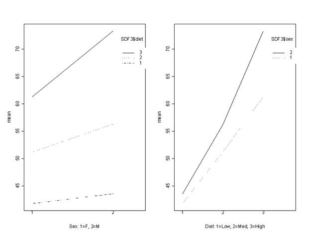
a. At the .10 level of significance, test for the presence of interaction

between Diet and Sex. Why did the result of the test turn out the way it

did? Use a PLOT of the means [plot can be done by hand] to explain why.

F_diet*sex = 41.2/13.42 = 3.071

F_0.10,2,12 = 2.81

Reject the F-test: 3.071>2.81. There is a significant interaction between diet and sex. It seems that the difference between male and females is greater for the high protein diet than it is for the low and moderate protein diets. The lines are not parallel.

b. At the .05 level of significance, test for the overall effect of Sex on

the mean weight gain. Why did the result of the test turn out the way it

did?--refer to your plot from [a] to answer this.

F_sex = 179.9/13.42 = 13.405

F_0.05,1,12 = 4.75, 13.405>4.75, reject the F statistic (p=0.003). There is a significant difference between the sexes—males have a greater weight gain (as seen by the plot of means).

c. At the .05 level of significance, test for the overall effect of the

three Diets on the mean weight gain. Why did the result of the test turn

out the way it did?--refer to your plot from [a] to answer this.

F_diet = 915.95/13.42 = 68.287

F_0.05,2,12 = 3.89, 68.287>3.89, reject the F statistic. There is a significant difference among the diet types—there is a consistent increase in weight gain as the level of protein in the diet gets higher, for both sexes.