QSCI 482/Prof. Conquest TAs Kennedy, Malinick, Norman
HW 6 - DUE FRIDAY, NOVEMBER 15, 2002

1. You have been hired as a statistial consultant to the Water Quality
Division of the Municipality of Metropolitan Seattle (METRO). (Even
though you only have one quarter of QSCI 381 and some weeks of QSCI 482, that puts you way ahead of a lot of other people!) METRO is going to be comparing two areas (one designated "polluted", one designated a
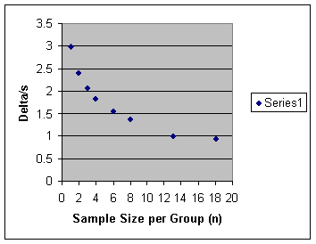
"reference control site") with respect to a number of measured responses like dissolved oxygen, turbidity, pH, and a number of toxicants(polyaromatic hydrocarbons, DDT, polychlorinated biphenyls, heavy metals, etc.) Since there are so many potential responses to consider, rather than focus on any one particular response, one way to have a sample size/power analysis discussion is to do a graph, with "delta/s" on the y-axis and "n per treatment group (assuming equal n's)" on the x-axis. Because of the expense involved, the sample sizes per area are going to be rather small, perhaps as low as 3 samples per area for either sediment samples or water samples! We're trying to show METRO the what happens statistically in terms of how the Minimum Detectable Effect changes as the number of samples per group changes. So, try out the values n = 3, 4, 5, 6, 8, 10, 15, 20 [that's the n *per group*], solve for the quantity "delta/s", and plot delta/s against n. Use alpha(2) = .10 and power = .90.

After you obtain your graph, what point would you emphasize to the METRO folks if you were doing a sample-size-power-analysis presentation? (A few sentences along with your graph. This means that you also have to turn in your graph.)

n	df	t 0.10 (2), 2(n-1)	t 0.10 (1), 2(n-1)	Delta/s
3	4	2.132	1.533	2.992
4	6	1.943	1.440	2.392
5	8	1.860	1.397	2.060
6	10	1.812	1.372	1.838
8	14	1.761	1.345	1.553
10	18	1.734	1.330	1.370
15	28	1.701	1.313	1.101
20	38	1.686	1.304	.946

Conclusions: Metro should be advised that initial increases in sample size per area (n) reap cost-effective benefits in terms of decreasing the standardized MDE. However, there are diminishing returns, so it may not be worth investing in additional samples beyond a certain n.

2. A soil scientist wants to see if the soil composition (having
something to do with the amount of carbon in the soil--the more carbon
in the soil, the darker the color) is different under two different
Treatments; denoted "T" and "C". Pairs of plots are located throughout a designated area (see notes p. 11-3 for a diagram). One member of each
pair is randomly assigned the "T" treatment and the other member of the
pair is assigned the "C" treatment. Now, the final measuring instrument
for amount of carbon in the soil is simply a SCORE between 0 and 100,
basedly largely on "carbon color observation" as described above.
Therefore, although a higher score represents "more carbon" than a lower score, the scientist is not sure that the scores are sufficiently exact to be treated numerically. Use a *nonparametric* test, then, to test whether the effects of the two treatments are the same, or whether they are different. You may use the .10 level of significance. The data are as follows:
Pair T C

1. 82 63
2. 69 42
3. 73 74
4. 43 37
5. 58 51
6. 56 43
7. 76 80
8. 65 82

What do you conclude?

We will do a Wilcoxon Signed Rank Test, which yields a T min of 9. The T crit. is T 0.10 (2), 9 = 5. Since T min is larger than the T critical, we fail to reject a null hypothesis (Ho) of no difference between treatments.

3. A random sample consisting of 11 automobile drivers was selected to see if alcohol affected time to complete a specific task. Each person's
response time was measured in a laboratory setting. Under one scenario, the person would drink a beverage that contained NO alcohol; under another scenario, the person would drink a beverage WITH alcohol. Treatments were randomized, and neither the drivers *nor* the people recording the test results knew which beverage actually contained the alcohol (this is known as a "double-blind" study). It is expected that the response time will *lengthen* when alcohol is consumed. The data (response time in seconds) are as follows:

SUBJECT NO ALCOHOL WITH ALCOHOL Di
1 7.1 7.4 0.3
2 6.3 6.2 -0.1
3 6.8 6.6 -0.2
4 8.4 9.3 0.9
5 6.9 7.2 0.3
6 8.5 8.8 0.3
7 7.3 7.6 0.3
8 7.7 7.9 0.2
9 8.1 8.7 0.6
10 7.4 7.9 0.5
11 6.6 7.0 0.4

d-bar = .318

s of d = .303

variance of d = .092

At the .10 level of significance, do a *parametric* test to see whether
the consumption of alcohol *increases* reaction time. What do you
conclude?

H₀: response time with alcohol is the same as with no alcohol;

H_a: response time with alcohol > response time without alcohol.

Data are normal and we perform a paired t- test.

t_0.10(1),10 = 1.372; Reject if t crit < t obs

t = (d-bar)/(S of d-bar) = 0.318/0.09127 = 3.486

1.372 < 3.486, so reject H₀. 0.0025 < p < 0.005

We have enough evidence to reject the null hypothesis and say that alcohol does increase the response time for automobile drivers doing specific tasks.