QSCI 482/Prof. Conquest TAs Kennedy, Malinick, Norman
HOMEWORK
4 - DUE
1. The following
data set is a sample of the corvina fish catch
(Sciaenideae) in the "primera" catch category, in kg/boat, from the
from the nonzero catches are lognormally distributed; that is, the
natural logarithms of the
catches follow a normal distribution.
Here are the original data (in kg/boat-trip):
28.7, 145.2, 18.0, 28.2, 7.9, 11.2, 7.4, 3.8, 26.9, 11.4,
6.6, 100.0,
17.8, 2.5, 5.8
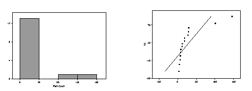
a. Using SPSS [or your favorite statistical software], do
[1] a
histogram of the data and [2] a
normal probability plot of the data.
Examine the histogram for symmetry and
"bell-shape" and any extreme
values; examine the normal probablity plot for normality. Give a brief
description of what each plot seems to show.
These data appear to be seriously non-normal. They are heavily asymmetric, right skewed, with a large
mode near zero and some data to the right.
The Q-Q plot shows a distinct departure from linearity. The concavity indicates skewedness.

b. Repeat the above (histogram and normal probability
plot) on the natural
logarithms of the data. What do
you conclude about the characteristics of
the data (catch vs. log catch), by looking at the graphs?
The plots of the new data appear to better approach
normality. The histogram appears fairly
bell-shaped and symmetric, and the QQ plot is close to linear. The log-transformation is definitely an
improvement of normality (although still not “perfect”).

2. Ocean Beauty Seafoods is
purchasing new batches of sardines from a
different supplier. Their
inspectors are not sure whether the average
length of the sardines from this
supplier are the same as or different
from the "old
standard" of 4.54 inches. A random sample of n=100 sardines
is drawn from the population,
giving a sample mean length of xbar=4.51
inches and a sample standard
deviation of s=.23 inches. (You may assume
that sardine lengths follow a
normal distribution.)
a. At the .05 level of significance, test to see whether
the mean length
of the new batches is different
from the "old standard" of 4.54 inches.
Include the P-value with your statistical results. What do you conclude?
H0: μ = 4.54; Ha: μ ≠
4.54. Data are normal, but σ is not
known, so use the t-distribution with 99 df.
|t0.05(2),99| = 1.984; Reject H0
if |t|>1.984
t=(4.51-4.54)/(0.23/sqrt(100)) =
-0.03/0.023 = -1.304
|-1.304|<1.984, fail to Reject H0: 0.10 < p
< 0.20
The mean length of the new batches is not significantly
different from the old standard.
b. Compute a 95% confidence interval for the population
mean sardine
length of the new batches.
Reconcile the result that you get for your
confidence interval with your answer to part (a) above.
95% CI: xbar+/-1.984*.23/sqrt(100) =
4.51+/-0.0456
4.46<=μ<=4.56
95% CI: (4.46,4.56)
Since the Confidence interval contains 4.54 and 95% of the
time our confidence interval contains the true mean, we cannot reject H0:
μ=4.54
3. A study of littleneck clams (Protothaca
staminea) was done in Garrison
Bay,
collected from a random sample
of 16 clams:
std. deviation s = 4.6 mm
n = 16 clams
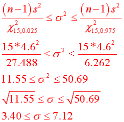
a. Compute a 95% confidence interval for the standard
deviation of the
population.

3b. For the littleneck clam
data, how large a sample is needed to reject
Ho: mu = 40.0 mm vs. Ha: mu not equal to 40.0 mm if in fact the *true
population mean* mu is really 38 mm? (Use s=4.6 mm, alpha = .10 for
variety, beta = .10.)
s=4.6 mm; s2 = 21.16, α = 0.10, β = 0.10; δ = 40-38 = 2.0; δ2
= 4.0;
s2/δ2 = 21.16/4 = 5.29
try n= ∞: n ≥ 5.29(1.645+1.282)2 =
45.32, round to 46
n=46: n ≥ 5.29(1.679+1.301)2 =
46.977, round to 47
n=47: n ≥
5.29(1.679+1.300)2 = 46.95, round to 47
Sample size n=47 is required.
4. Scientists have conducted studies on the reproductive
toxicity effects
of Nitrofen,
an herbicide used for weed control in rice and other grains.
Nitrofen is persistent in
aquatic systems. Its reproductive toxicity
effects were tested on Cladocera dubia (a zooplankton)
at a certain
concentration.
a. Suppose we want to compare these data to a *documented
standard control
value* of mu=32.0.
Even before running the experiment, enough has been
known about Nitrofen
to suspect that if Nitrofen does anything at all to
C. dubia, it should *decrease*
the average number of offspring.
Assuming normality of the data (or at least regarding the
behavior of
the sample mean), do a test at
the alpha = .10 level to see if there has
been a decrease in the average
number of offspring when compared with the
standard control value of 32.0.
Be sure to write down the null and
alternative hypotheses. Include
the P-value associated with your test
statistic.
The data for this part (3a) are as follows: for each of
10 animals, the
number of offspring was
recorded, yielding a sample average of 28.3
offspring and a sample standard
deviation of s=3.6 offspring.
What do you conclude as a result of your test?
H0: μ ≥ 32.0; Ha: μ
< 32.0. Data are normal, but σ
is not known, so use the t-distribution with 9 df.
t0.10(1),9 =
1.383; Reject if t<-1.383
t = (28.3-32)/(3.6/sqrt(10)) =
-3.7/1.138 = -3.25
-3.25 < -1.383, so reject H0. p ~ 0.005
We have enough evidence to say that Nitrofen
does decrease the number of offspring of Cladocera dubia relative to the control value of
32.
b. If we want to achieve 95% power to test the null and
alternative
hypotheses as in part (3a)
above, what kind of minimum detectable effect
would we be able to detect
statistically? Use alpha = .10, n=10, and use
3.6 as the standard deviation.
α = 0.10; df = 9; β =
0.05; s = 3.6; t0.10(1),9 =
1.383; t0.05(1),9 = 1.833
δ = 3.6/sqrt(10) *
(1.383+1.833) = 1.138*3.216 = 3.66