Draft; January 1998
by Brian T.R. Lewis and LeRoy M. Dorman
Typical seafloor noise spectra in the range .01 to 10 Hz.
Microseisms; A relationship between sea-surface swell and sea-floor noise
A comparison of noise on basalt and sediment covered sea-floor .
During the NOBS experiment in 1991 seismic noise in the frequency range .01 to 10 Hz was measured with arrays of pressure and velocity (seismometer) sensors on sedimented seafloor and seafloor composed of basalt. Wave height data were recorded simultaneously on FLIP.
We find a distinct correlation between sea-surface wave amplitude at about 0.1 HZ and seafloor pressure and velocity at frequencies of about 0.2 Hz (the microseism band) . In this band the seafloor noise tracks the sea-surface wave amplitude at twice the frequency of the waves and the ratio between vertical velocity and pressure is controlled by the compliance of the seafloor. The more compliant sediment-covered seafloor produces larger amplitude vertical velocity noise than the basalt seafloor. This noise propagates at phase velocities of greater than 1 km/sec and is consistent with non-linear wave interaction theory for the generation of this noise.
At frequencies above about 1 Hz the noise on the seismometers is dominated by interface waves propagating in a low velocity channel associated with the ocean to seafloor transition (Stonely waves). This noise propagates at speeds less than about 0.1 km/sec and it's characteristics are determined by the seafloor and the transition from a zero rigidity ocean to a high rigidity lithosphere. Seafloor having thick transition regions with shear velocities less than 1.5 km/sec have a spectral peak on the seismometers at a lower frequency than regions with a thin transition region. Pressure sensors appear to be unaffected by the nature of the seafloor.
Several experiments and theoretical analyses have shown that sea-floor noise in the frequency range .01 to 10 Hz is from three sources. At very low frequencies (.01 HZ) gravity waves on the sea-surface produce sufficient pressure disturbance at the seafloor to contribute to seafloor noise (Crawford et al 1991). At frequencies near 0.1 HZ the non- linear interaction of swells at the sea-surface produce acoustic waves at twice the frequency of the generating swells (Webb et al 1992). These acoustic waves propagate as Rayleigh waves which are coupled into the sub-sea-floor. At frequencies above 1 HZ noise on the sea-floor appears to be dominated by Stoneley waves which are produced at the sea-floor by, for example, scattering of acoustic waves generated at the sea-surface (e.g. breaking waves) and by biologic activity. The Stoneley waves propagate in the zone at the interface between the ocean and the sea-floor where the shear velocity is less than the compressional wave velocity of the water. Because the shear velocity is usually very low the speed of these waves is very low and therefore the wavelength is very short. Tuthill et al 1981, Dougherty and Stephen 1988, Schreiner et al 1990, Dorman et al 1993, Liu et al 1993, Park and Odom 1997.
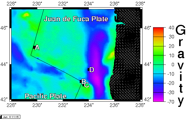
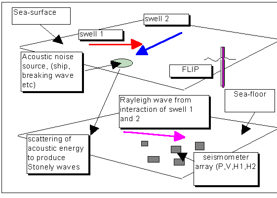
Because the sea-floor in the deep ocean can vary widely from low rigidity mud to high rigidity basalt it is expected that the displacement component of the sea-floor noise would depend on the rigidity of the sea-floor. To test this hypothesis an experiment was undertaken in 1991. In the experiment four arrays of seismometers were set on sea-floor where the sediment had thicknesses of approximately 0, 10, 100 and 1000 meters. In addition the R/V Flip was deployed near one of the arrays to record swell height and wind, as well as other environmental factors. This was a unique opportunity as it is usually very difficult to have measurements of swell concurrent with measurements of sea- floor noise. The NE Pacific Ocean off the coast of Oregon was chosen as the site because of the opportunity to realize all the desired sea-floor types within a small geographic area on and near to the Juan de Fuca ridge system, Figure_1 . The general hypotheses being tested are shown schematically in figure 2 .
In this paper we will use the data to examine the general properties of sea-floor noise, the relationship between swell and sea-floor noise, the properties of sea-floor noise at frequencies above 1 HZ, and finally the variation of sea-floor noise with sediment thickness.
A description of the instrumentation may be found in Jacobson et al 1991
The locations of the seismic instruments are given below.
Array A . Juan de Fuca Ridge. 0 m sediment
57 -130.2226 44.9512 2296
54 -130.2226 44.9468 2296
Array B. Blanco fracture zone. 10 m sediment
2 -126.3853 42.8390 2700
5 -126.3751 42.8409 2690
6 -126.3766 42.8368 2655
9 -126.3833 42.8429 2685
13 -126.3813 42.8430 2700
53 -126.3815 42.8417 2690
55 -126.3808 42.8428 2690
58 -126.3800 42.8405 2690
61 -126.3813 42.8377 2690
Array C. Flank. 100 m sediment
1 -126.6032 43.0241 3125
4 -126.5934 43.0217 3125
51 -126.5915 43.0253 3125
52 -126.5960 43.0272 3125
56 -126.5985 43.0245 3125
59 -126.5937 43.0292 3125
60 -126.5997 43.0282 3125
62 -126.5972 43.0220 3125
63 -126.5977 43.0255 3125
64 -126.5947 43.0252 3125
Array D. Cascadia Basin. 1000 m sediment.
Also site of R/V FLIP
7 -125.9976 43.6964 3025
8 -125.9729 43.6968 3025
10 -125.9801 43.7101 3025
11 -125.9947 43.7008 3025
12 -125.9843 43.7058 3025
14 -125.9834 43.6960 3025
15 -125.9879 43.7103 3025
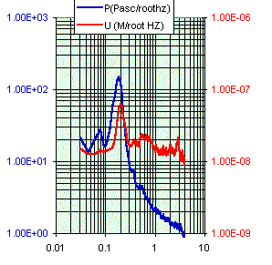
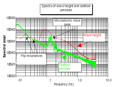
When we compare typical sea-floor noise records of pressure and displacement (obtained by correcting the velocity measurement) we see that they are similar at the low frequency end, .01 to .3 HZ. but diverge above .3 HZ. , with the displacement becoming increasingly larger than the pressure. This can be seen in Figure 3 , which shows typical sea-floor noise recorded on a hydrophone and a vertical seismometer. There is also a well defined peak in the noise at 0.2 HZ. This is the so-called microseism peak.
The relationship between pressure and displacement for a plane acoustical wave incident at the sea-floor is defined by the impedance equation P=-2*pi*i*rho*f*Uz, where rho is the density, f is the frequency and Uz the displacement. Note that we would expect from this relation that the pressure divided by the displacement would increase linearly with frequency. The data in figure 3 shows the opposite trend. This suggests that we are not dealing simply with incident plane waves, and that a more complicated wave propagation is involved.
This paper will show that the properties of the microseism peak are consistent with Rayleigh wave propagation in the ocean and sub-sea-floor and attempt to show that the displacement noise becomes larger at higher frequencies in relation to the pressure because of Stonely wave propagation at the sea-floor interface.
It is now widely held that the microseism peak in sea-floor noise is caused by swell at the sea-surface, Webb 1992. Swells at the sea-surface interact non-linearly to produce an acoustic wave at twice the frequency of the interacting swells. This acoustic wave then propagates in the ocean-seafloor wave guide as a Rayleigh wave. The data we obtained in this experiment confirms this hypothesis.
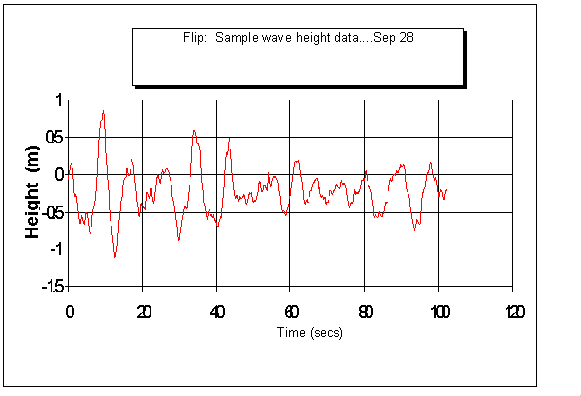
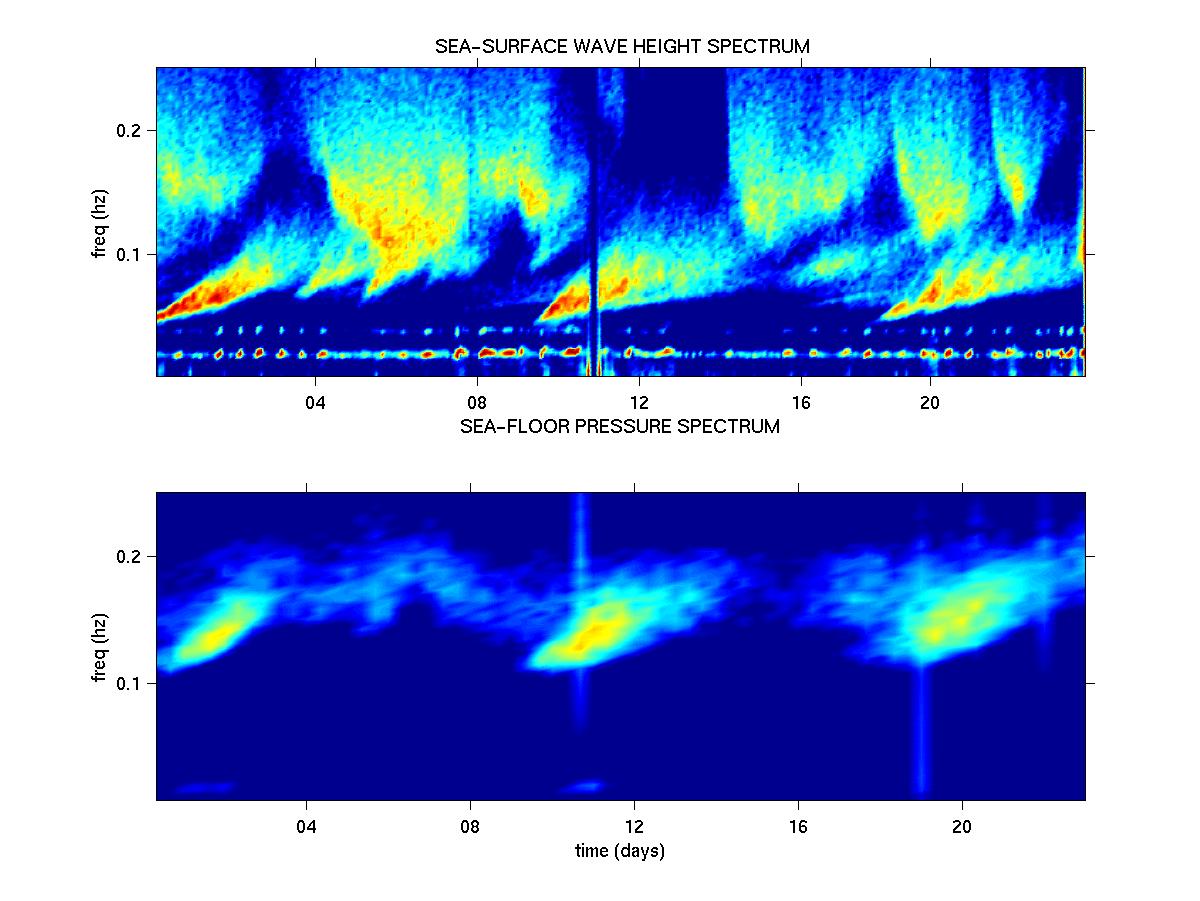
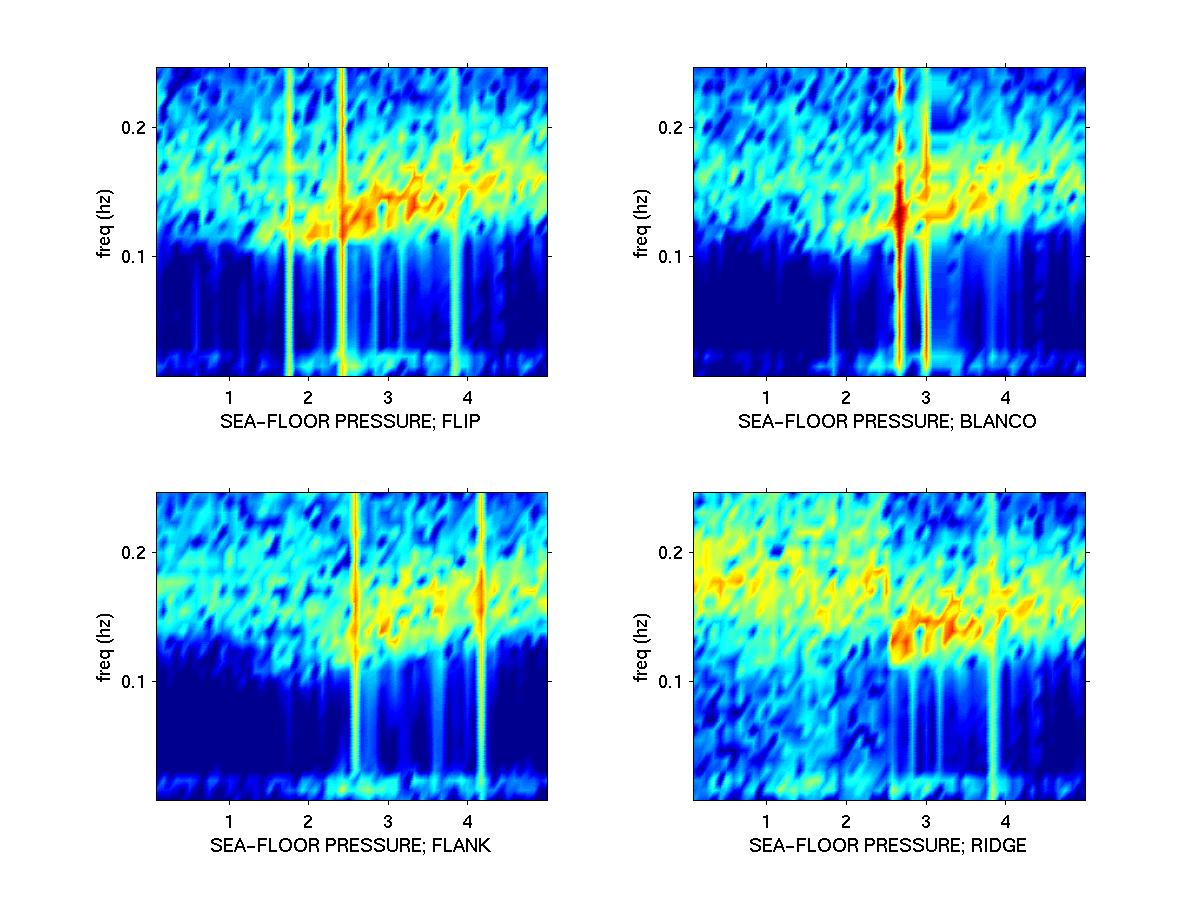
Wave height data were recorded on FLIP throughout the NOBS experiment, a sample of these data is shown in Figure 4 . Spectra of the wave height data are compared to sea-floor pressure in Figure 5 and we see clearly that there is a peak in the wave data at about 10 sec. period and a peak in the sea-floor pressure at about 5 sec. period. To show that these two peaks are causally related we compared the wave and sea-floor pressure data for a 24 day period to see if increases in wave height associated with storm activity are related to increase in microseism noise at the sea floor. That they are related can be clearly seen in Figure 6 , a spectrogram of wave height and sea-floor noise for 24 days at the FLIP site. These data show that the sea-floor noise is closely related to the wave height in time. Stated another way, the sea-floor noise at a particular site is closely related to the sea-state of the ocean surface immediately above the sea-floor site. Spectrograms from the other array sites show similar increases in noise levels at about the same time as the FLIP site, indicating that the storm events are producing similar effects at the other sites. See Figure 7 ,a comparison of spectrograms from all 4 sites during one noise event.
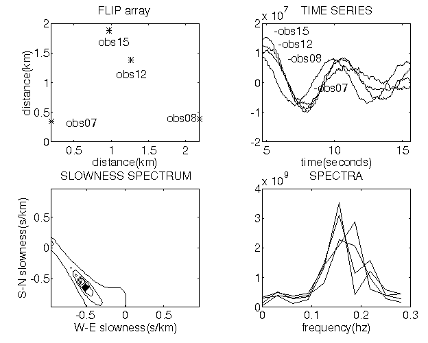
So far the data clearly show that there is a peak in the sea-floor noise at twice the frequency of the sea-surface swells and that they are closely correlated in time. By inference it is highly likely that the sea-floor noise is causally related to the swell. To show that the sea-floor noise is propagating as Rayleigh waves in the ocean sea-floor wave guide we need to demonstrate that the noise has phase velocities of order of a few km/sec. In principle this can be done by using phase delays between array elements. In practice the array size (or inter-element spacing) can limit the resolution of this measurement. In this experiment inter-element spacings were a few hundred meters, based on a desire to resolve short wavelength phenomena, and not optimal for wavelengths of several km. In spite of this low resolution velocity estimates can be made using 3 dimensional frequency- wavenumber (f-k) spectra.
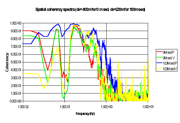
To estimate usable f-k spectra requires that the coherence between array elements be high at the frequency of interest (0.2 HZ for microseisms). Figure 8 shows examples of spatial coherency between pairs of seismometers at each array site. We see that coherency is high at 0.2 HZ and inter-element spacings of a few hundred meters for all the sites. We also see that the coherency drops off rapidly at higher frequencies and is low at 0.1 HZ.
Estimates of the f-k spectra for the FLIP site are shown in Figure 9 These spectra of the microseism noise show the horizontal phase velocity to be about 1.5 km/sec at 0.2 HZ. and direction of propagation to be from the South West. This result is consistent with Rayleigh wave propagation.
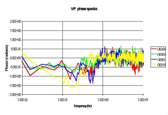
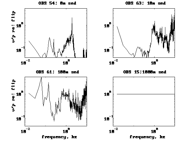
Because the non-linear interaction of short wavelength swells at the sea-surface results in long wavelength acoustic waves in the ocean we will expect these acoustic waves to have properties similar to plane waves at the sea-floor. One of these properties, determined from the impedance relationship P=-2*pi*i*rho*f*Uz , involves a 90 degree phase shift between the pressure and displacement. Figure 10 shows vertical/pressure phase spectra for all sites. For the FLIP site, which has the largest sediment thickness (about 1000 meters) , the phase shift is close to 90 degrees. For the other sites with smaller sediment thickness the phase shifts are progressively smaller as the sediment thickness decreases, suggesting that the sea-floor properties are effecting the microseismic noise characteristics.
Based on the phase velocity of the sea-floor microseismic noise and the coherence between the swells and this noise it seems reasonable to conclude that the microseismic noise is indeed caused by the local swell action and that the noise is propagating as Rayleigh waves in the ocean-seafloor wave guide.
In the previous section we have shown that the microseismic noise at about 0.2 HZ. is characterized by relatively high phase velocities (1.5 km/sec), which correspond to wavelengths of about 7 km, and as a consequence high coherence between seismometers a few hundred meters apart. We also noted in the previous section that the coherence fell dramatically above 1 HZ. This implies that the noise above 1 HZ is of wavelength less than a few hundred meters. It must therefore have phase velocities less than about 100- 200 m/sec and must be propagating in a mode much different from the microseismic noise.
Because the coherence above 1 HZ is so low we cannot use the array data to measure the velocity of the noise in this band directly. We are able, however, to use bottom shots to show that there is an energetic phase generated by the shots which propagates at a very slow phase velocity. This is the well known Stoneley wave and it propagates in the waveguide formed by the mud and other low shear strength materials at the interface between the water and the sea-floor. Its speed is mostly determined by the shear speed of the interface material. Tuthill et al 1981, Schreiner and Dorman 1990 and others have shown other experimental evidence for this wave. Park and Odom 1977, show that this wave is very efficiently generated and propagated by scattering at the sea-floor.
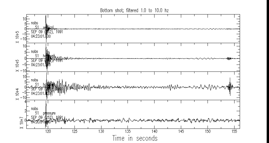
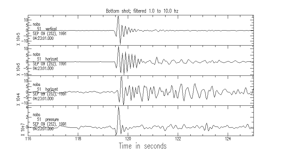
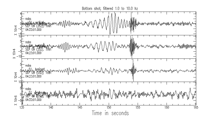
As already mentioned the lack of coherence is the primary evidence in this experiment that this noise is propagating as Stoneley waves. Bottom shots add data supporting this inference. As an example Figure 11 shows the direct and Stoneley waves from a bottom shot as recorded at one OBS . The considerable time delay between the direct arrival and the Stoneley wave indicates its slow speed. An enlargement of the direct arrival from the bottom shot is shown in Figure 12 and an enlargement of the Stoneley wave from the bottom shot is shown in Figure 13 .
We see from Figure 13 that the Stoneley wave has its largest amplitude on the vertical seismometer and is not visible on the pressure sensor. This explains why the sea-floor noise on the vertical seismometer increases relative to the pressure sensor as frequency increases above 1 HZ. (see figure 3).
These bottom shot data are evidence that disturbances at the sea-floor are capable of energizing this waveguide. Other sources of stimulus would be animals and acoustic waves scattered by irregularities at the sea-floor.
There is also evidence from this experiment that the characteristics of both the microseismic noise and the Stoneley wave noise are dependent on the properties of the sea-floor. This evidence comes from comparing the noise spectra of the pressure and vertical seismometer sensors.
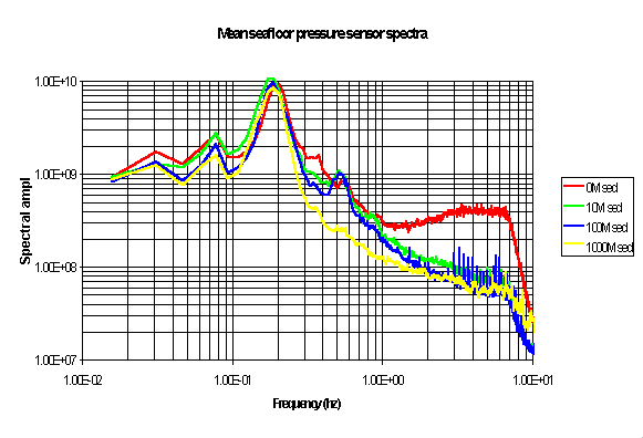
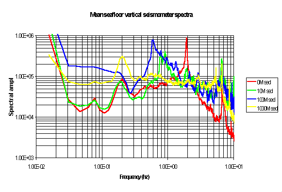
Figure 14 shows mean sea-floor pressure spectra from all sites. Figure 15 shows mean sea-floor vertical seismometer spectra from all sites. These spectra were estimated by taking the mean of many adjacent and non-overlapping spectra. From these two figures it is clear that the pressure spectra are much less dependent on sea-floor properties than the vertical seismometer spectra. There is an unusual peak at about 2 HZ. on the pressure sensor at the zero sediment site. This site was on the axis of the Juan de Fuca ridge and the noise could be due to hydrothermal sources.
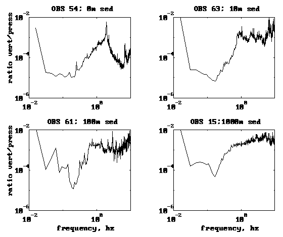
To characterize the dependence of the noise on site properties (primarily sediment thickness) we have calculated ratio spectra for all four sites by dividing the vertical seismometer spectra by the pressure spectra, Figure 16 . These ratio spectra were then normalized to the FLIP site on the basis that the FLIP site had the thickest sediment and most closely approximated a situation in which the velocity only varied with depth. Figure 16b shows V/P ratio spectra for all 4 sites as referenced to the FLIP site.
These ratio spectra suggest that sediment thickness has an effect on sea-floor in at least two ways. The first relates to microseismic noise. The ratio spectra show that the sites with thin sediment have V/P ratios about 10 times less than the FLIP site. This can be understood in terms of the compliance of the sea-floor in response to long wavelength forcing. For sites with thick sections of low strength sediments the sea-floor has a greater displacement response than a site with no or little sediment. See Crawford et al 1991 for more information. The second effect of the sea-floor on noise is at frequencies above 1 HZ. The ratio spectra data show a peak near 1 HZ which generally becomes smaller and moves to progressively lower frequencies as the sediment thickness increases. At the FLIP site the peak is almost absent and it is largest on the sites with little sediment. This suggests the possibility of a resonance effect related to the thickness of the sediments. Webb 1992 has quantitatively analysed this situation in terms of mode excitation and dissipation.
A principle goal of this experiment was to determine if sea-floor noise was dependent on the nature of the sea-floor, hence the name of the experiment, Noise on Basalt and Sediment (NOBS). The data from this experiment show clearly that sea-floor noise is dependent on the details of the physical properties at the sea-floor.
For microseismic noise propagating as Rayleigh waves in the ocean-sea-floor waveguide at about 0.2 HZ the compliance of the sea-floor effects the amplitude of the displacement of the sea-floor. Sites with lower compliance will have greater displacement due to the swell generated noise.
Noise above 1 HZ is very sensitive to the properties of the sea-floor. A low shear strength layer at the sea-floor permits efficient propagation of very slow Stoneley waves. Resonance effects appear to be possible and related to the details of the layer at the sea- floor. Sites with thin sediment layers appear to be more noisy at 1 HZ than sites with a thick layer of sediment.
This experiment was supported by the Office of Naval Research under contracts N00014- 90-1881 and N00014-91-j-1336 under the Marine Geology and Acoustics Programs
Olga Ingerman helped greatly with the data analysis.
Crawford, W.C., S.C. Webb and J.A. Hilderbrand, Seafloor compliance observed by long- period pressure and displacement measurements: J.Geophys.Res., 96,16151-16160, 1991
Dorman,L.M, Schreiner,A.E, Bibee,L.D., and Hiderbrand,J.A., 1993, Deep-water seafloor array observations of seismo-acoustic noise in the eastern Pacific and comparisons with wind and swell, in B. Kerman, Ed., Natural Physical Sources of Underwater Sound, Cambridge, England, Kluwer,.
Dougherty M.E. and R.A Stephen, Seismic energy partitioning and scattering in laterally heterogeneous ocean crust. PAGEOPH, 128, 195-229, 1988.
Jacobson,R.S., Dorman,L.M., Purdy,G.M.,Schultz,A., and Solomon,S.C., Ocean Bottom Seismometer facilities Available, EOS, Trans. of AGU, 72,506-515. 1991.
Liu, J., Schmidt,H. and Kuperman, W.A., Effect of a rough seabed on the spectral composition of deep ocean infrasonic ambient noise: J. Acoust.Soc.Am., 93, 753-769, 1993.
Park, M., and Odom, R.I., The effect of stochastic rough interfaces on coupled-mode elastic waves. Submitted to Geophysical Journal International July 30, 1997.
Schreiner,A.E. and Dorman,L.M., Coherence lengths of seafloor noise: Effects of seafloor structure: J.Acoust.Soc.Am, 88, 1503-1514. 1990.
Tuthill,J.D., Lewis, B.T.R., and Garmany,J.D., Stoneley waves, Lopez Island noise and deep sea noise from 1 to 5 Hz: Mar. Geophys.Res., 5, 95-108, 1981
Webb, S.C. The equilibrium oceanic microseism spectrum, J. Acoust. Soc. Am. 92(4), 2141-2158, 1992
Figure 1 Location of the seismic arrays
Figure 2 A schematic of the hypotheses being tested
Figure 3 Typical sea-floor noise recorded on a hydrophone and a vertical seismometer.
Figure 4 Sample wave height data as recorded by FLIP
Figure 5 A comparison of spectra of wave height and sea-floor pressure
Figure 6 Spectrogram of wave height and sea-floor noise for 24 days at the FLIP site
Figure 7 A comparison of spectrograms from all 4 sites during one noise event.
Figure 8 Spatial coherency between pairs of seismometers at each array site.
Figure 9 Frequency wavenumber spectra of the microseism noise showing the velocity and direction of propagation
Figure 10 Vertical/pressure phase spectra for all sites showing 90 degree phase shift for microseism noise.
Figure 11 A bottom shot as recorded at one OBS showing the direct and Stoneley waves.
Figure 12 An enlargement of the direct arrival from the bottom shot.
Figure 13 An enlargement of the Stoneley wave from the bottom shot.
Figure 14 Mean sea-floor pressure spectra from all sites
Figure 15 Mean sea-floor vertical seismometer spectra from all sites.
Figure 16 V/P ratio spectra for all 4 sites.
Figure 16b V/P ratio spectra for all 4 sites as referenced to the FLIP site.
Brian T.R.Lewis
University of Washington, WB-10
School of Oceanography
Seattle, WA, 98195
LeRoy M. Dorman
University of California
Scripps Inst. of Oceanography
La Jolla, Ca. 92093