The eig(A) command

A = [1, 3; 3, 1];
eig(A)

		ans =

    			-2
    			 4

[V,D] = eig(A)

		V =

   			-0.7071    0.7071
    			0.7071    0.7071


		D =

    			-2     0
     			0     4

A*V(:,1) - D(1,1)*V(:,1)

		ans =

     			0
     			0

A*V(:,2) - D(2,2)*V(:,2)

		ans =

     			0
     			0

Complex eigenvalues

A = [0, 1;-1,0];
eig(A)

		ans =

   			0.0000 + 1.0000i
   			0.0000 - 1.0000i

[V,D] = eig(A)

		V =

   			0.7071 + 0.0000i   0.7071 + 0.0000i
   			0.0000 + 0.7071i   0.0000 - 0.7071i


		D =

   			0.0000 + 1.0000i   0.0000 + 0.0000i
   			0.0000 + 0.0000i   0.0000 - 1.0000i

A*V(:,1) - D(1,1)*V(:,1)

		ans =

     			0
     			0

A*V(:,2) - D(2,2)*V(:,2)

            ans =
                          0
                          0

Spectral factorization ($A = S\Lambda S^{-1}$)

A = [1, 3; 3, 1]; % a symmetric matrix
[V,D] = eig(A)

		V =

   			-0.7071    0.7071
    			0.7071    0.7071


		D =

    			-2     0
     			0     4

V*D*V'

		ans =

    		1.0000    3.0000
    		3.0000    1.0000

A

		A =

     			1     3
     			3     1

QR eigenvalue algorithm

A = [1, 3; 3, 1];
for i = 1:10
    [Q,R] = qr(A);
    A = R*Q;
end

A

		A =

    			4.0000    0.0059
    			0.0059   -2.0000

eig(A)

		ans =

    			4.0000
   			-2.0000

A = [1, 3, 1; 3, 0, -1; 1,  -1, 1]
for i = 1:100
    [Q,R] = qr(A);
    A = R*Q;
end
A

		A =

     			1     3     1
     			3     0    -1
     			1    -1     1


		A =

    			3.5475    0.0000    0.0000
    			0.0000   -3.0340    0.0000
    			0.0000   -0.0000    1.4865

eig(A)

		ans =

    			3.5475
   			-3.0340
    			1.4865

Singular values

Suppose we have a rectangular matrix, which of course won't have eigenvalues.  Is there an analog to eigenvalues for rectangular matrices?  Consider the eigenvalues of $A^TA$ and $AA^T$.  These will be called Singular Values.

A = randn(20,10);
[U,S,V] = svd(A);

norm(U*S*V' - A)

		ans =

   			1.8299e-14

Using the SVD for image compression

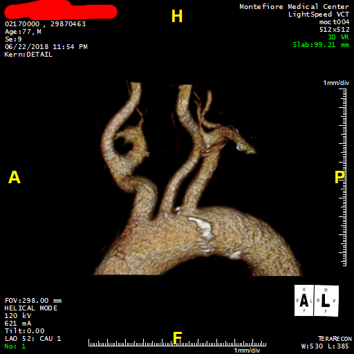
A = imread('image.png');
A = rgb2gray(A);
imshow(A)

For this image, the first singular value is dominant.

[U,S,V] = svd(double(A));
S(1:5,1:5)

		ans =

   			1.0e+04 *

    				1.9457         0         0         0         0
         			0    1     .3044         0         0         0
         			0              0    0.7280         0         0
         			0              0         0    0.6954         0
         			0              0         0         0    0.6415

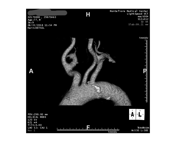
If we reconstruct the image using only the first singular value, we get a surprisingly good idea what the picture is.

k = 1; % A = U S V^T
W = V';
[m,n] = size(A);
B =  U(:,1:k)*S(1:k,1:k)*W(1:k,:);
B = uint8(B);
imshow(B)
fprintf('Compression ratio = %.5f', (m*k+k+n*k)/(m*n))

		Compression ratio = 0.00391

This required less then 1% of the storage required to store the full matrix.

Next, we look at the size of the singular values, relative to the top singular value:

DiagS = diag(S);
for i = 1:length(S)
if DiagS(i)/DiagS(1) < 0.05
i
break
end
end

		i =

    			55

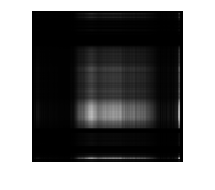
The 55th singular value is less than 5% of the magnitude of the top singular value. So, we will chop there and see what image we reconstruct.

W = V';
[m,n] = size(A);
B =  U(:,1:i)*S(1:i,1:i)*W(1:i,:);
B = uint8(B);
imshow(B)
fprintf('Compression ratio = %.5f', (m*i+i+n*i)/(m*n))

		Compression ratio = 0.21505

With just over 20% of the storage, we can compress the image so that it is at least recognizable. There are some issues that affect the true amount of storage. These are related to the fact that the original image was an integer matrix and $U,V,S$ are now double precision numbers. Whether justified, or not, we ignore that here for simplicity.