Bonus Coding Lecture
A word on underdetermined systems
We are trying to solve
however for both the over and underdetermined problems we don't have a
solution. For overdetermined systems, the nice thing is the
problem
is the closest equation to have a solution. For underdetermined problems we again consider
, but this time
is singular. So we have to do
and that will give you your least squares solution. This works if
is invertible, which for our case it is. In the case where
is not invertible there are other techniques such as using SVD.
In summary, use
Parallel Computing
Here is an example of a Beuwolf supercomputing cluster. Most
supercomputers are much more sophisticated than this these days, but
this is an easier illustration.
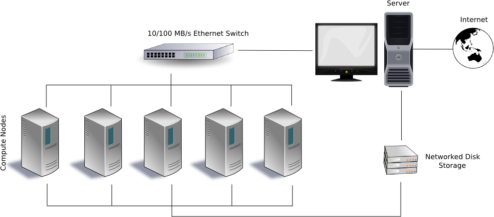
With any type of supercomputing cluster, the key ingredient is message
passing, which unfortunately creates overhead, so for small problems a
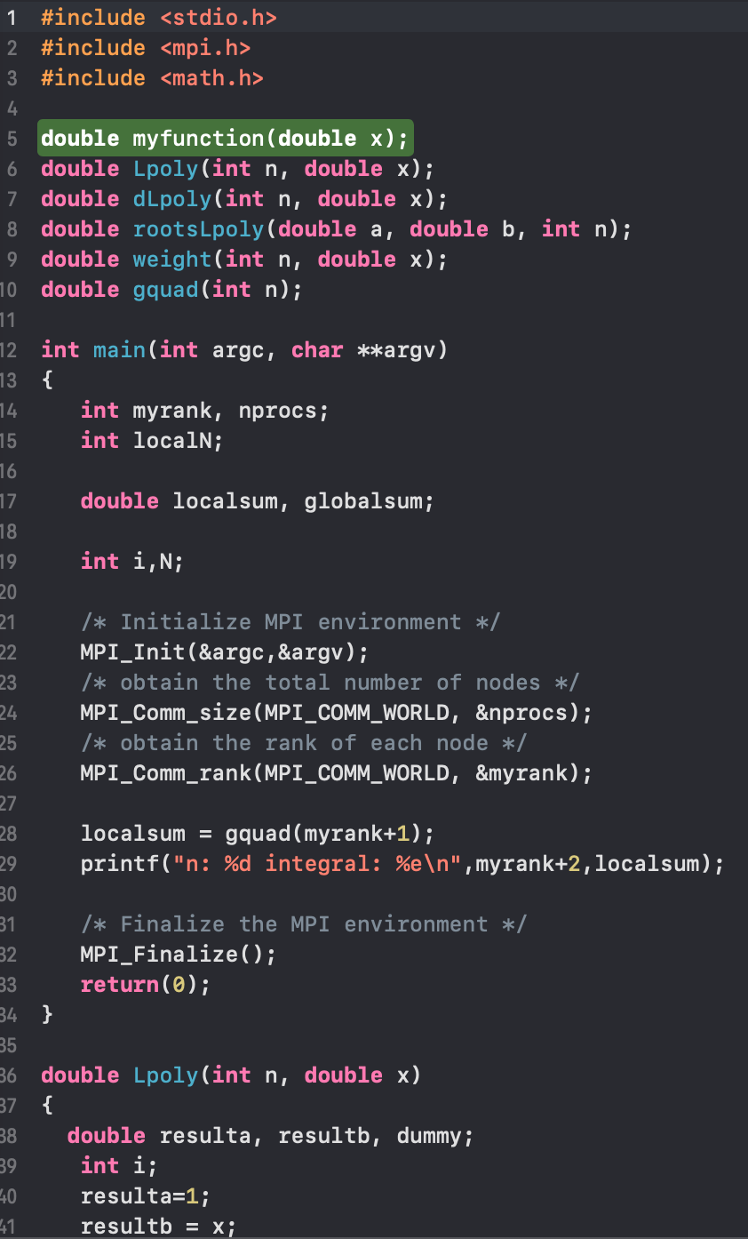
parallel code will always be slower. On the C programming language
this is done using the
Message Passing Interface (MPI). Below is one of my codes from
years ago using MPI to implement Finite Differences to solve Partial
Differential Equations. I still use MPI to solve equations (often
via Finite Element Methods), but these days it's usually the grad
students that work with me doing the implementing. Things are
simplified in MATLAB, and we can use the parfor command, which is part
of the parallel computing toolbox. The parallel computing toolbox
is usually standard, and I believe you can use the onine version of
MATLAB through UW, but if anyone doesn't have it or can't access it, let
me know.
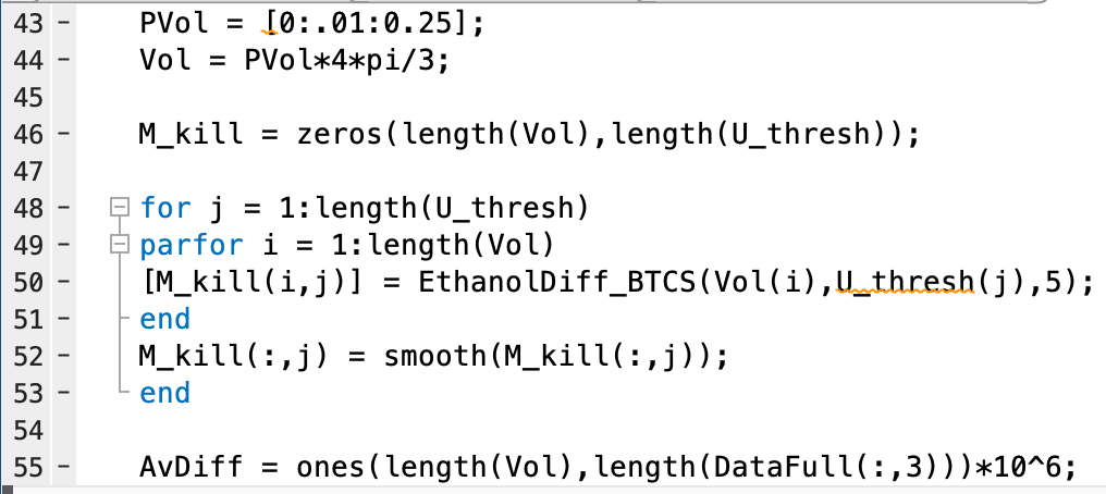
Here is a more recent code I wrote on MATLAB that uses Finite Differences to solve one of my Partial Differential Equations models that describes the spread of a drug through a tumor. I use parfor to distribute the Finite Differences code to various computing units (nodes), then in the current code the nodes pass their results to the main node, which is then used to couple my drug dynamics model with my population dynamics to simulate a predictive model of drug response.
Jacobi's Algorithm
Recall Jacobi's Algorithm: $ A\vec x = \vec b$ $ (L + D + U) \vec x = \vec b$ $ D^{-1}( L + D + U) \vec x = D^{-1}\vec b$ $ \vec x + D^{-1}(L + U) \vec x = D^{-1} \vec b$
Then apply the Neuman series iteration with $M =
- D^{-1}(L + U)$ and $\vec b$ replaced with $D^{-1} \vec b$.
When we did this last time we actually optimized the linear multiplication, however if we did not do any optimization we would get the following code:
function [y] = LinearJacobi(y,A,b)

L = tril(A,-1);
U = triu(A,+1);
D = diag(diag(A));

c = inv(D)*b;

y = -inv(D)*(L + U)*y + c;
Now lets try to parallelize this by noticing we can do each row
multiplication on a different computing unit. We use parfor on MATLAB
in order to distribute the work to all of our computing units. I have a
fairly old laptop which only has two cores, so mine only gets
distributed to two computing units. You have may have a nicer (perhaps
gaming?) laptop with more cores, and you'll notice much better
performance than mine.
function [y] = ParallelJacobi(y,A,b)

L = tril(A,-1);
U = triu(A,+1);
D = diag(A);

FirstTermMultiplication = -(L + U)*y;

parfor i = 1:length(b)
    y(i) = FirstTermMultiplication(i)/D(i) + b(i)/D(i);
end
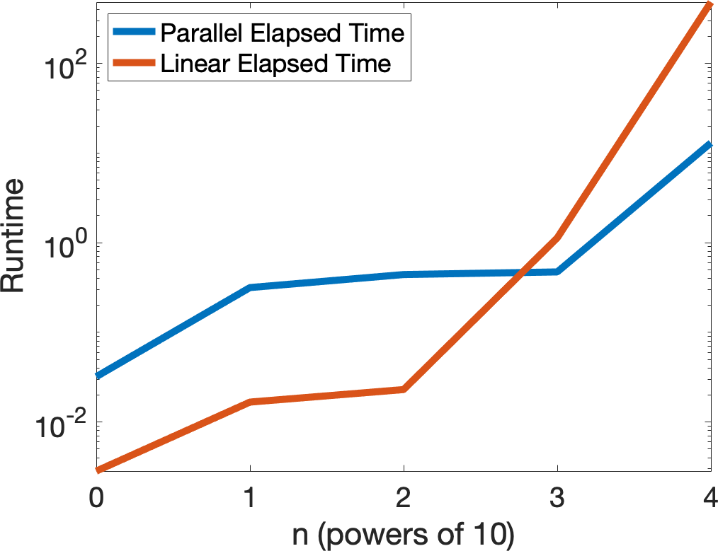
Now lets compare the two algorithms.
ParallelTime = 0*[0:4];
LinearTime = ParallelTime;

for n = 0:length(ParallelTime)-1

A = diag([1:10^n]) + .01*randn(10^n);
b = ones(length(A),1);

y= zeros(length(b),1);

E = 1e-8;

tic
while max(abs(A*y - b)) > E
    y = ParallelJacobi(y,A,b);
end
ParallelTime(n+1) = toc;


y= zeros(length(b),1);

tic
while max(abs(A*y - b)) > E
    y = LinearJacobi(y,A,b);
end
LinearTime(n+1) = toc;

end

set(0,'defaultAxesFontSize',20)
semilogy([0:length(ParallelTime)-1],ParallelTime,[0:length(ParallelTime)-1],LinearTime,'Linewidth',5)
xlabel('n (powers of 10)')
ylabel('Runtime (log scale)')
legend('Parallel Elapsed Time','Linear Elapsed Time','Location','northwest')